
|
|
|
|
|
|
|---|---|---|---|---|---|
 |
|---|
 |
 |
 |
|---|---|---|
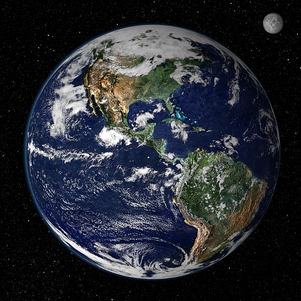
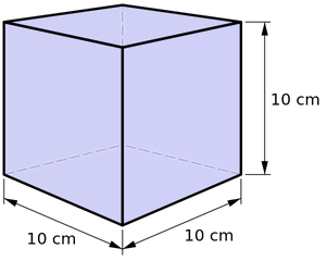
The fundamental mechanical units are the meter, second, and kilogram. They were defined in 1793 as the "Standard International" (SI) units, or "MKS" units.
Quantity   Unit        Definition

Length     Meter       The Earth's circumference is 40 million meters
Time       Second      There are 86400 seconds in one Earth day
Mass       Kilogram    The mass of a cube of water 10 cm on a side is 1 k
 |
 |
 |
|---|---|---|
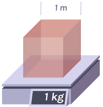
Density of water =1000 kg/meter = 1 g/cm Density of air = 1.2 kg/meter = .0012 g/cm
 |
 |
 |
 |
 |
 |
|---|---|---|---|---|---|
 |
 |
 |
 |
 |
 |
 |
|---|
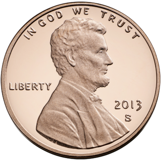
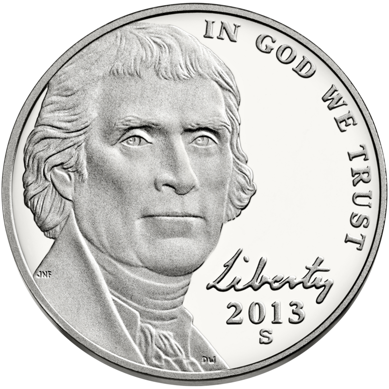
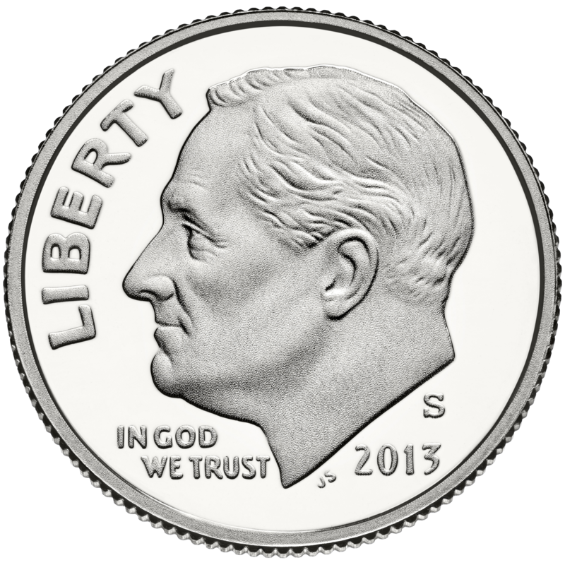
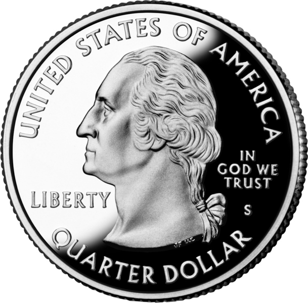
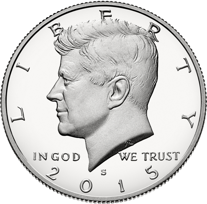
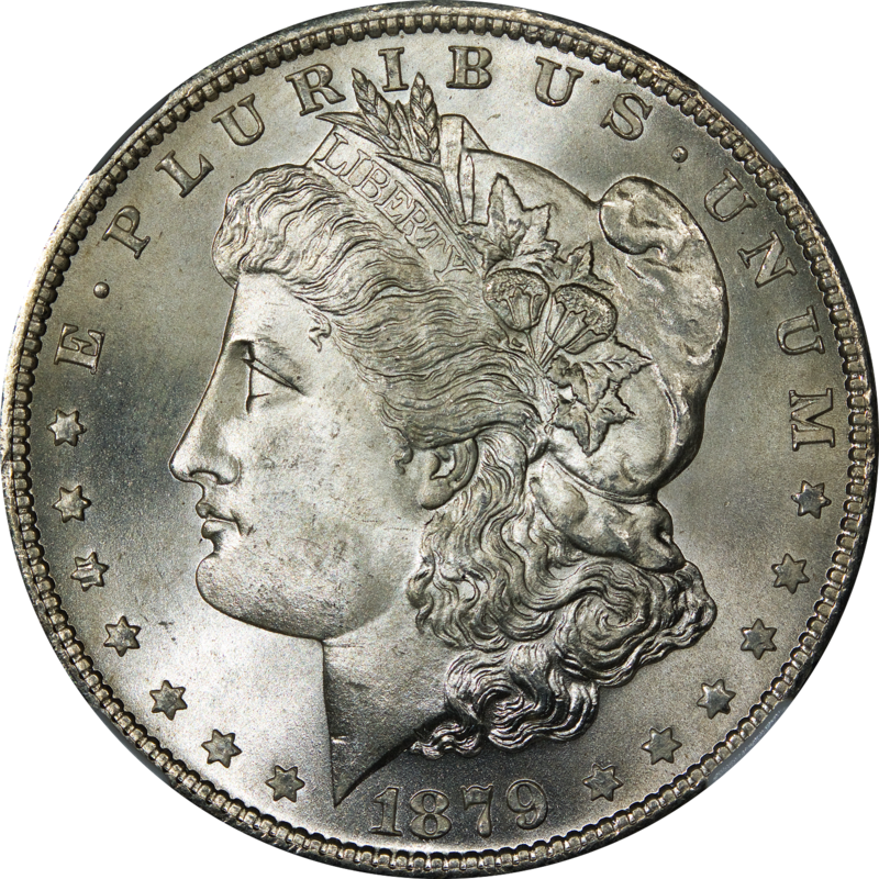
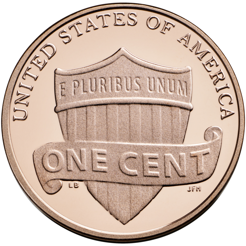
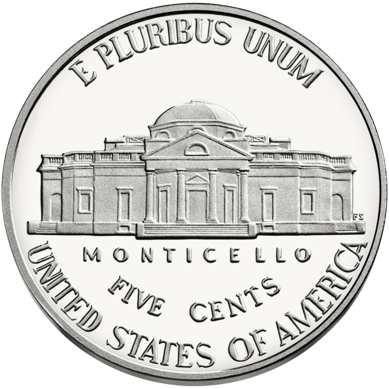
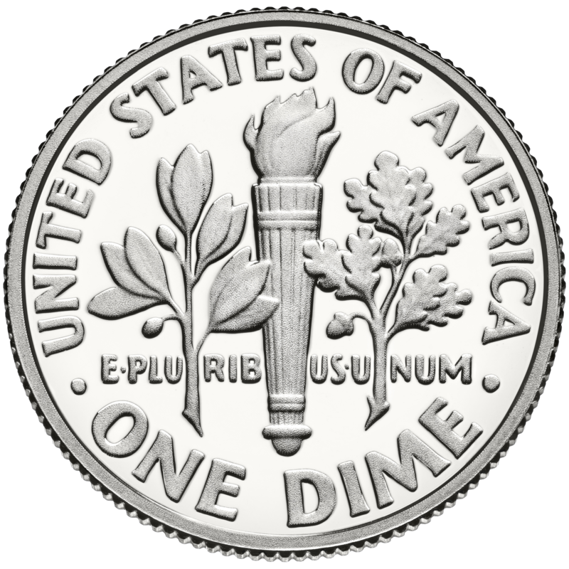
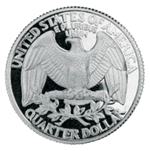
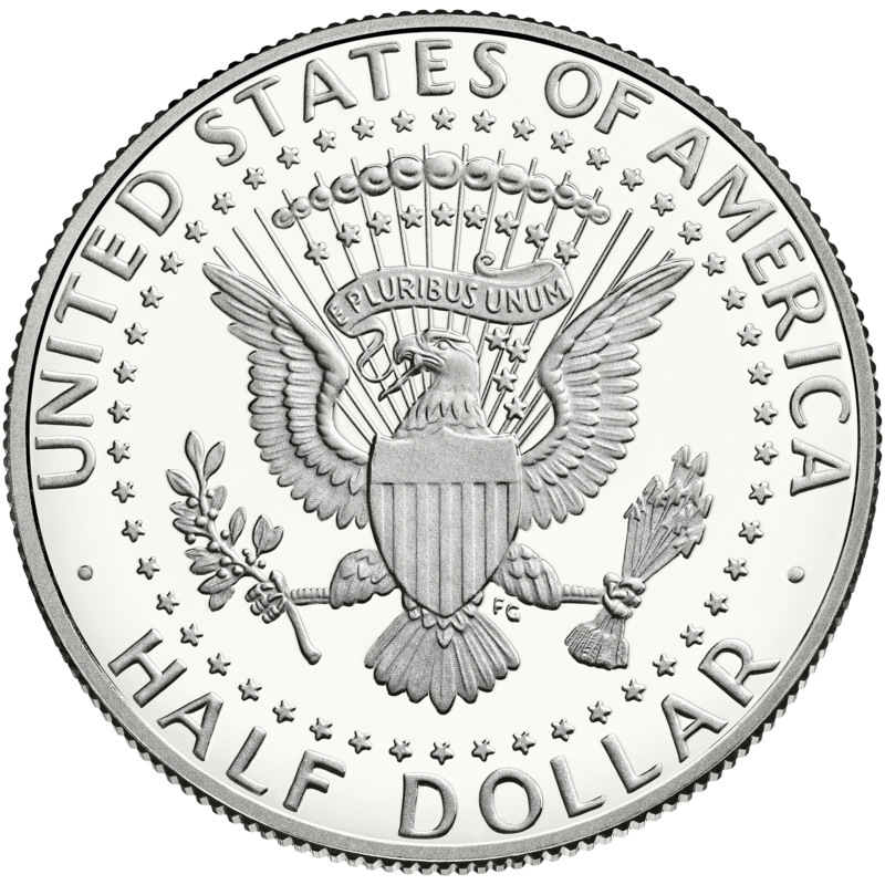
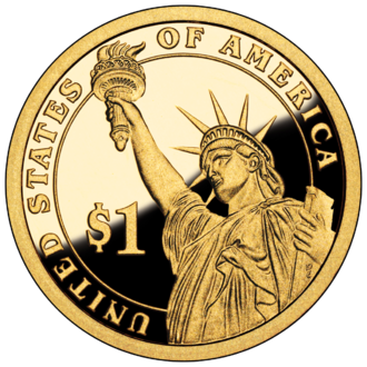
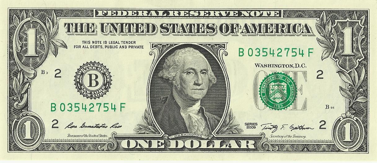
             Mass   Diameter  Thickness  Density  Copper  Nickel  Zinc  Manganese
             (g)      (mm)      (mm)

Dime         2.268   17.91      1.35      8.85    .9167   .0833
Penny        2.5     19.05      1.52      7.23    .025            .975         Copper plated
Nickel       5.000   21.21      1.95      7.89    .75     .25
Quarter      5.670   24.26      1.75      9.72    .9167   .0833
1/2 dollar  11.340   30.61      2.15     10.20    .9167   .0833
Dollar       8.100   26.5       2.00      9.73    .885    .02     .06   .035   Plated with manganese brass
Dollar bill  1.0    155.956      .11       .088                                Height = 66.294 mm
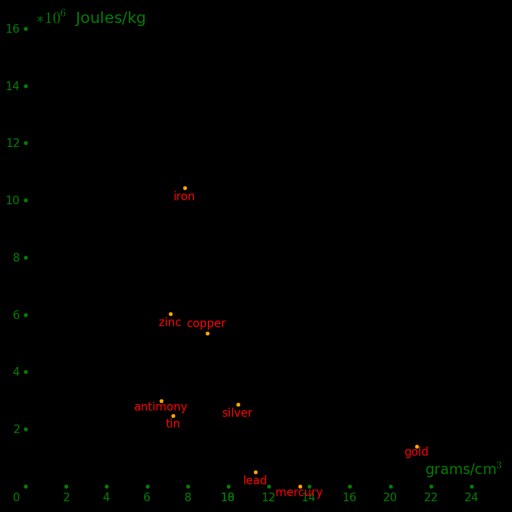
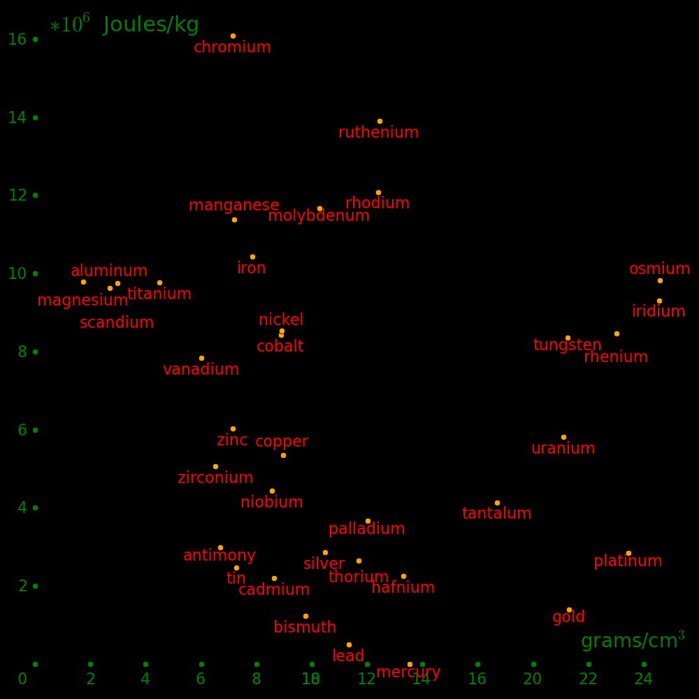
In ancient times, gold was an ideal currency because it was hard to counterfeit. No other element known had a density that was nearly as large.
Silver can be counterfeited because lead is more dense and cheaper.
The metals known to ancient civilizations were:
         Density    Known to ancient
         (g/cm3)    civilizations

Zinc       7.1       *
Manganese  7.2
Tin        7.3       *
Iron       7.9       *
Nickel     8.9
Copper     9.0       *
Bismuth    9.8       *
Silver    10.5       *
Lead      11.3       *
Mercury   13.5       *
Tungsten  19.2
Gold      19.3       *
Platinum  21.4
Osmium    22.6                Densest element
In ancient times, gold could be countereited to a limited degree because mass
and volume could not be measured precisely. One could shave a small amount of
gold from a coin, small enough so that the change in volume is undetectable.
Once tungsten was discovered in 1783 it became easy to counterfeit gold.
Newton was Master of the Mint and he placed the United Kingdom on the gold standard. He was the Sherlock Holmes of his era and he caught all the counterfeiters.
 |
|---|
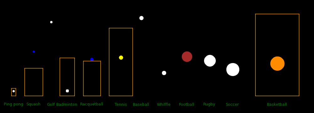
In this figure, ball sizes are in scale with each other and court sizes are in scale with each other. Ball sizes are magnified by 10 with respect to court sizes.
The distance from the back of the court to the ball is the characteristic distance the ball travels before losing half its speed to air drag.
             Ball    Ball   Court   Court    Ball
           diameter  Mass   length  width   density
             (mm)    (g)     (m)     (m)    (g/cm3)

Ping pong      40      2.7    2.74    1.525   .081
Squash         40     24      9.75    6.4     .716
Golf           43     46                     1.10
Badminton      54      5.1   13.4     5.18    .062
Racquetball    57     40     12.22    6.10    .413
Billiards      59    163      2.84    1.42   1.52
Tennis         67     58     23.77    8.23    .368
Baseball       74.5  146                      .675   Pitcher-batter distance = 19.4 m
Whiffle        76     45                      .196
Football      178    420     91.44   48.76    .142
Rugby         191    435    100      70       .119
Bowling       217   7260     18.29    1.05   1.36
Soccer        220    432    105      68       .078
Basketball    239    624     28      15       .087
Cannonball    220  14000                     7.9     For an iron cannonball
 |
 |
|---|---|
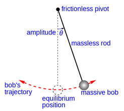
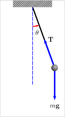
Construct a pendulum that is 1 meter long and measure its period for small oscillations using a phone clock.
Vary the oscillation angle and plot the period as a function of oscillation angle.
Measure the period for small oscillations for a pendulum with lengths of .5, 1, and 2 meters.
P½  =  Period for a length of .5 meters
P1  =  Period for a length of 1 meters
P2  =  Period for a length of 2 meters
Using the measured values, calculate P1/P½, P2/P1, and P2/P½.
The analytic result for the period for small oscillations is:
Pendulum length  =  L  =  1 meter
Gravity          =  g  =  9.8 m/s2
Period           =  T  =  2 π (L/g)1/2  =  2.006 seconds
The oscillation period increases as the angle increases.
Era             Method for measuring speed

Renaissance     Use a pendulum clock to measure time and a ruler to measure distance
20th century    Use a pocket watch or phone clock to measure time and a ruler to measure distance
21st century    Film the object and analyze the video frame-by-frame
Roll a ball across a table and measure its speed using the stopwatch and the phone video methods. What would you estimate is the error for each method?
Velocity  =  V
Time      =  T
Position  =  X  =  V T
By viewing a video frame-by-frame you can measure the position and time of the ball for a set of different times. For example,
Frame   Time   Position
         (s)      (m)

  0      .0      .10
 12      .5      .21
 24     1.0      .32
 36     1.5      .43
 48     2.0      .54
 60     2.5      .65
 72     3.0      .76

Frame rate = 24 frames/second
The velocity at Time=.75 can be approximated as:
Time of first measurement      =  T1  =  .5
Time of second measurement     =  T2  = 1.0
Position at first measurement  =  X1  =  .21
Position at second measurement =  X2  =  .32
Time difference                =  T  =  T2 - T1  =  1.0 - .5  =  .5
Position difference            =  X  =  X2 - X1  =  .32 - .21 =  .11
Velocity at Time=.75           =  V  =  X  / T   =  .22 meters/second
 |
|---|
Roll two balls toward each other so that they collide head-on and rebound in the opposite direction, and use a phone video to measure the quantities listed below.
Blue ball:  Initially on the left  and moving to the right
Red ball:   Initially on the right and moving to the left

Momentum       =  Mass * Velocity
Kinetic energy =  ½ * Mass * Velocity2


Mass of blue ball             =  M1
Mass of red ball              =  M2
Initial velocity of blue ball =  V1i
Initial velocity of red ball  =  v2i
Final velocity of blue ball   =  V1f
Final velocity of red ball    =  v2f
Initial momentum of blue ball =  Q1i  =  M1 V1i
Initial momentum of red ball  =  Q2i  =  M2 V2i
Final momentum of blue ball   =  Q1f  =  M1 V1f
Final momentum of red ball    =  Q2f  =  M2 V2f
Initial energy of blue ball   =  E1i  =  ½ M1 V1i2
Initial energy of red ball    =  E2i  =  ½ M2 V2i2
Final energy of blue ball     =  E1f  =  ½ M1 V1f2
Final energy of red ball      =  E2f  =  ½ M2 V2f2
Total initial momentum        =  Qi   =  Q1i  +  Q2i
Total final momentum          =  Qf   =  Q1f  +  Q2f
Total initial energy          =  Ei   =  E1i  +  E2i
Total final energy            =  Ef   =  E1f  +  E2f
Energy ratio                  =  Er   =  Ef   /  Ei
Momentum is conserved in collisions: Initial momentum = final momentum.
Collisions usually convert some energy to heat: Final energy < Initial energy
 |
 |
|---|---|
Gravity energy  =  Mass * g * Height
Kinetic energy  =  ½ * Mass * Velocity2
Drop a ball from rest and measure the height of the first bounce.
Ball mass              =  M
Gravity constant       =  g  =  9.8 meters/second2
Initial height         =  Xi
Final height           =  Xf       (Maximum height after the first dim
Initial gravity energy =  Ei  =  M g Xi
Final gravity energy   =  Ef  =  M g Xf
Height ratio           =  Xr  =  Xf / Xi
Energy ratio           =  Er  =  Ef / Ei
Plot the height ratio (Xr) as a function of height (Xi).
Suppose you climb a set of stairs.
Height  =  Height of a set of stairs
Mass    =  Mass of a person
Gravity =  9.8 m/s2
Energy  =  Mass * Gravity * Height
Time    =  Time required to climb the stairs
Power   =  Energy / Time
        =  Mass * Gravity * Height / Time
        =  Mass * Gravity * Vertical velocity
Agility =  Power / Mass
Climb 3 flights of stairs and measure the above quantities.
If a 100 kg person eats 3000 Calories in one day then
Energy  =  3000 Calories * 4.2e3 Joules/Calorie
        =  12.6 MJoules
Power   =  Energy / Time
        =  12.6e6 Joules / 1 Day
        =  12.6e6 Joules / 86400 seconds
        =  146 Watts or Joules/second
Agility =  Power / Mass
        =  1.46 Watts/kg
Measure your maximum running speed and calculate your kinetic energy.
Mass           =  Mass of a person
Velocity       =  Maximum running velocity
Kinetic energy =  ½ Mass * Velocity2
g              =  9.8 meters/second2
Gravity energy =  Mass * g * Height
Kinetic energy =  ½ Mass * Velocity2
How much gravitational potential energy does it take to raise an object vertically from the surface of the Earth to a height of 400 km (the height of the space station)?
The space station orbits at 7.8 km/s. How much kinetic energy does 1 kilogram of matter have if it is moving at this speed?
Using Wikipedia, how much energy does one kilogram of gasoline have?
If an object starts from rest at X=0 and undergoes constant acceleration then after time T,
Time         =  T
Acceleration =  A
Velocity     =  V  =  A T
Position     =  X  =  .5 A T2  =  V2 / (2 A)

Velocity      =  Change in position  /  Change in time
Acceleration  =  Change in velocity  /  Change in time
Record a video of a ball dropping and measure the height (X) and time (T) to reach the floor. Calculate the gravitational acceleraton. Use X=.5 meters and 2.0 meters.
A = 2 X / T2
.gif) |
 |
|---|---|
Roll a sphere down an inclined plane and measure the distance traveled for the first 4 seconds. Let
X1  =  Distance traveled after 1 second
X2  =  Distance traveled after 2 seconds
X3  =  Distance traveled after 3 seconds
X4  =  Distance traveled after 4 seconds
If the acceleration is constant then
R2  =  X2/X1  =  4
R3  =  X3/X1  =  9
R4  =  X4/X1  = 16
Measure X1, X2, X3, X4, and calculate R2, R3, R4.
 |
|---|
Construct a pendulum using as large a length and mass as possible. The Earth's rotaton causes the pendulum to precess like the animation above, although the precession is exaggerated in the animation.
Start the pendulum and observe its direction anle and then observe the direction angle one hour later.
Q  =  Rate of change of the direction angle of a pendulum
   =  360 * sin(Latitude)        degrees/day
   =  360 * sin(40.667 degrees)  degrees/day                 For New York City
   =  234.6                      degrees/day
   =    9.78                     degrees/hour

New York City Latitude   =  40.667 degrees North
New York City Longitude  =  73.933 degrees West
100 Zhang Heng constructs a seismometer using pendulums that was capable of
detecting the direction of an Earthquake.
1500 Pendulums are used for power for machines such as saws, bellows, and pumps.
1582 Galileo finds that the period of a pendulum is independent of mass
and oscillation angle, if the angle is small.
1636 Mersenne and Descartes find that a pendulum is not quite isochronous.
Its period increased somewhat with its amplitude.
1656 Huygens builds the first pendulum clock, with a precision of
15 seconds per day. Previous devices had a precision of 15 minutes per day.
1658 Huygens publishes the result that pendulum rods expand when heated.
This was the principal error in pendulum clocks.
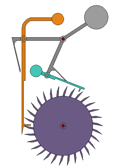
1670 Previous to 1670 the verge escapement was used, which requires a large angle.
The anchor escapement mechanism is developed in 1670, which allows for a smaller
angle. This increased the precision because the oscillation period is
independent of angle for small angles.
1673 Huygens publishes a treatise on pendulums.
1721 Methods are developed for compensating for thermal expansion error.
1726 Gridiron pendulum developed, improving precision to 1 second per day.
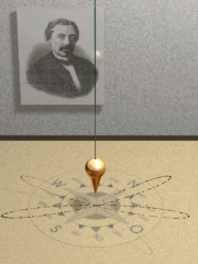
1851 Foucault shows that a pendulum can be used to measure the rotation period of
the Earth. The penulum swings in a fixed frame and the Earth rotates with
respect to this frame. In the Earth frame the pendulum appears to precess.
1921 Quartz electronic oscillator developed
1927 First quartz clocks developed, which were more precise than pendulum clocks.
 |
|---|
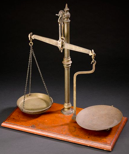
Construct a balance scale using any materials that would have been available to Newton.
Collect a set of identical coins to use as standard masses. Dimes are ideal because they have the smallest mass.
Measure the mass of one of the balls from the list below in units of coin masses and then use the table of coins to convert it to kg. What is the relative error?
Suppose there are N coins on the left side of the balance and N+1 coins on the right, with all coins being identical. If N is small then the scale can tell the difference and if N is large it can't. What is the largest value of N for which you can tell the difference between N coins and N+1 coins?
We can define a "resolution" for the scale as 1/N. For example, if a scale has a maximum mass of 1 kg and it can resolve down to 1 gram, then its resolution is .001 kg / 1 kg = 0.001.
For a nickel, measure the mass, diameter, and thickness, and calculate the volume and density. Compare it to the table below.
Volume   =  Thickness * π * (Diameter / 2)2

Density  =  Mass / Volume
 |
|---|
Dot size  =  Atomic radius
          =  (AtomicMass / Density)1/3
For gases, the density at boiling point is used.
        Earliest   Shear    Melt  Density
        known use  Strength (K)   (g/cm3)
        (year)     (GPa)
Wood    < -10000     15        -    .9
Rock    < -10000
Carbon  < -10000
Diamond < -10000    534     3800   3.5
Gold    < -10000     27     1337  19.3
Silver  < -10000     30     1235  10.5
Sulfur  < -10000
Copper     -9000     48     1358   9.0
Lead       -6400      6      601  11.3
Brass      -5000    ~40                    Copper + Zinc
Bronze     -3500    ~40                    Copper + Tin
Tin        -3000     18      505   7.3
Antimony   -3000     20      904   6.7
Mercury    -2000      0      234  13.5
Iron       -1200     82     1811   7.9
Arsenic     1649      8     1090   5.7
Cobalt      1735     75     1768   8.9     First metal discovered since iron
Platinum    1735     61     2041  21.4
Zinc        1746     43      693   7.2
Tungsten    1783    161     3695  19.2
Chromium    1798    115     2180   7.2


Stone age    Antiquity
Copper age    -9000
Bronze age    -3500
Iron age      -1200
Carbon age     1987       Jimmy Connors switches from a steel to a graphite racket
Bronze holds an edge better than copper and it is more corrosion resistant.
 |
|---|
Horizontal axis:  Density
Vertical axis:    Shear modulus / Density       (Strength-to-weight ratio)
Strength-to-weight ratio is important for swords. Iron makes a better sword than copper or bronze.
 |
|---|
Horizontal axis:  Density
Vertical axis:    Shear moduus / Density       (Strength-to-weight ratio)
Beryllium is beyond the top of the plot.
Metals with a strength-to-weight ratio less than lead are not included, except for mercury.
 |
|---|
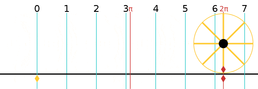
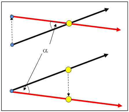
= Angle in radians (dimensionless) X = Arc distance around the circle in meters (the red line in the figure) R = Radius of the circle in meters X = R
 |
 |
|---|---|
π is defined as the ratio of the circumference to the diameter.
Full circle = 360 degrees = 2 radians 1 radian = 57.3 degrees 1 degree = .0175 radians Angle in degrees = (180/π) * Angle in radians Angle in radians = (π/180) * Angle in degrees
 |
|---|
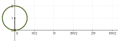
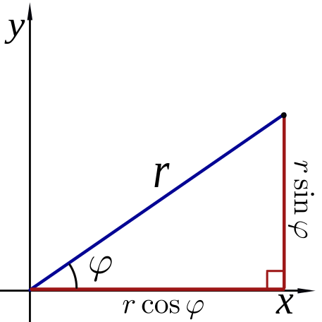
Radius = R Angle = (radians) X coordinate = X = R cos() Y coordinate = Y = R sin()
Let (X,Y) be a point on a circle of radius R.
θ   =  Angle of the point (X,Y) in radians
X   =  R cos(θ)
Y   =  R sin(θ)
Y/X =    tan(θ)
If θ is close to zero then
X ~ R
Y << X
Y << R
sin(θ) ~ θ
tan(θ) ~ θ
The "small angle approximation" is
Y/X ~ θ
 |
|---|
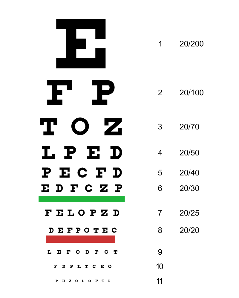
A person with 20/20 vision can distinguish parallel lines that are spaced by an angle of .0003 radians, about 3 times the diffraction limit. Text can be resolved down to an angle of .0015 radians.
Distance from the eye to the letter  =  X
Height of the letter                 =  Y
Resolution angle                     =  A  =  X/Y        (You can use the small-angle approximation)


        Resolution     Resolution    Diopters
        for parallel   for letters   (meters-1)
        lines          (radians)
        (radians)
20/20     .0003         .0015          0
20/40     .0006         .0030         -1
20/80     .0012         .0060         -2
20/150    .0022         .011          -3
20/300    .0045         .025          -4
20/400    .0060         .030          -5
20/500    .0075         .038          -6
"Diopters" is a measure of the lens required to correct vision to 20/20.
The units that optometrists use (20/X) are goofy. A more sensible unit is to define a scaled resolution.
Measured resolution angle          =  A
Resolution angle for 20/20 vision  =  a  =  .0003  radians
Scaled resolution                  =  S  =  A/a
The closest distance your eyes can comfortably focus is 20 cm. If a computer screen is at this distance then the minimum resolvable pixel size is
Pixel size = Angle * Distance = .0003 * .2 = .00006 meters = .06 mmFor a screen that is 10 cm tall this corresponds to 1670 pixels. This is referred to as a "retinal display".
Measure your visual resolution angle for the following situations:
Resolving pairs of dots
Resolving parallel lines
Resolving Letters (both for dim and bright light)
Resolving pixels on a phone
All waves diffract, including sound and light. Light passing through your pupil is diffracted and this sets the limit of the resolution of the eye.
Diameter of a human pupil = D = .005 meters Wavelength of green light = W = 5.5*10 meters Characteristic diffraction angle = θ = .00013 radians = 1.22 * W/D (for a circular aperture)
 |
 |
|---|---|
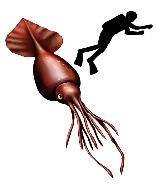
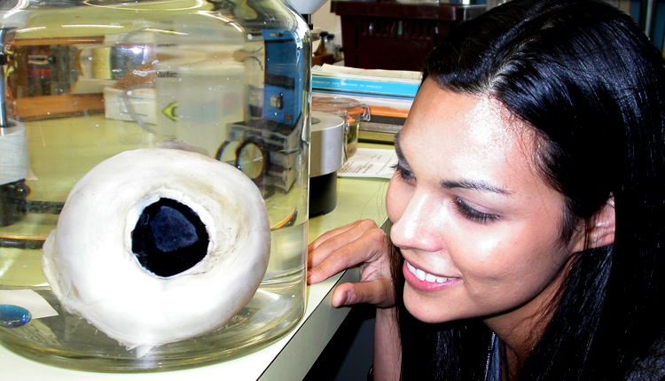
The colossal squid is up to 14 meters long, has eyes up to 27 cm in diameter, and inhabits the ocean at depths of up to 2 km.
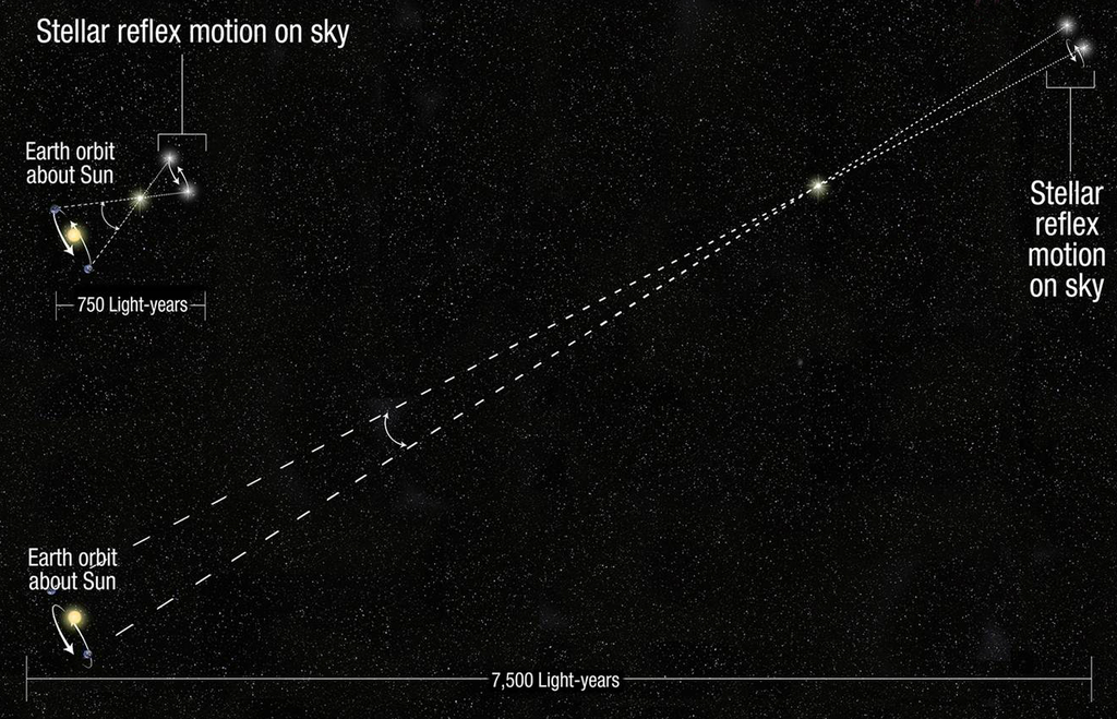
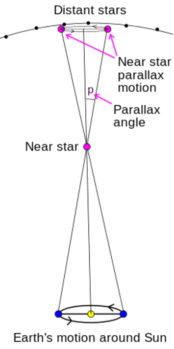
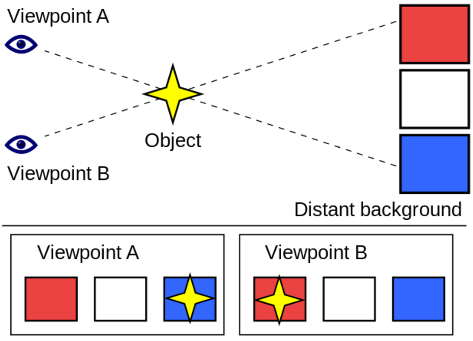
There are two ways to measuring parallax: "without background" and "with background". The presence of a background improves the precision that is possible.
Without background:
 |
 |
 |
|---|---|---|
With background:
 |
 |
 |
|---|---|---|
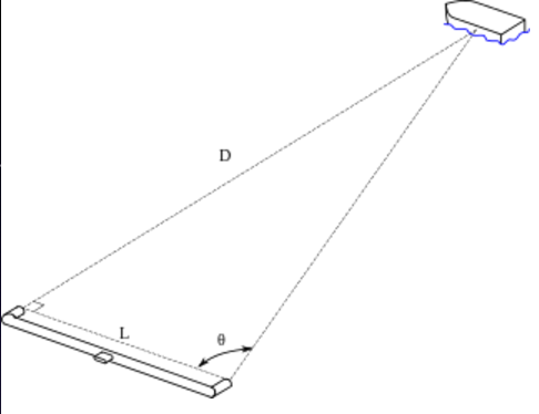
Place two observer marks on the floor around 1 meter apart and place a target mark on the other side of the room, at least 8 meters away from the observer marks. Arrange the observer marks to be perpendicular to the target mark, like in the figure above.
X  =  Distance between the observer marks
D  =  Distance from an observer mark to the target mark
      (should be the same for both observer marks)
 |
 |
|---|---|
Align the flat end of a protractor with the line between the observer marks, and measure the angles from the observer marks to the target mark. Both angles should be near 90 degrees.
θ1  =  Angle from observer mark #1 to the target mark
θ2  =  Angle from observer mark #2 to the target mark
θ  =  |θ2 - θ1|
Using the small angle approximation,
θ = X / Dwhere θ is in radians. Measure X and θ and calculate D with the small-angle approximation. Also measure D.
Look out the lab window and find two buildings that overlap each other. The far building should be much further away than the near building. Use Google Maps to find the distances to the buildings.
The near building is the target for which we will measure the distance, and the far building is the background that allows us to measure precise angles.
Select two vantage points from inside the lab that are as far apart as possible and that can both see the buildings, and measure the distance between them. Measure the difference in the angle that the two vantages perceive of the near building, and calculate the distance to the near building.
Distance to near building = Distance between the vantage points / Difference in angle
 |
|---|
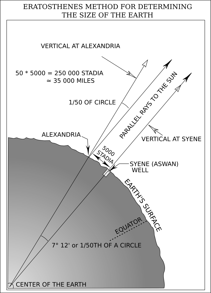
Eratosthenes produced a measurement of the Earth that was accurate to 2 percent.
 |
 |
|---|---|
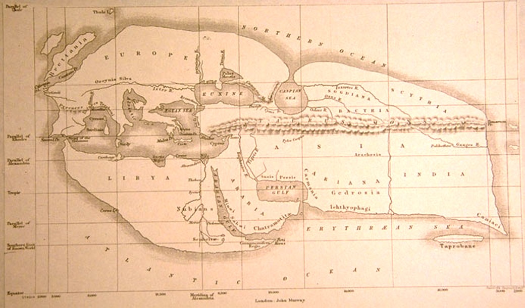
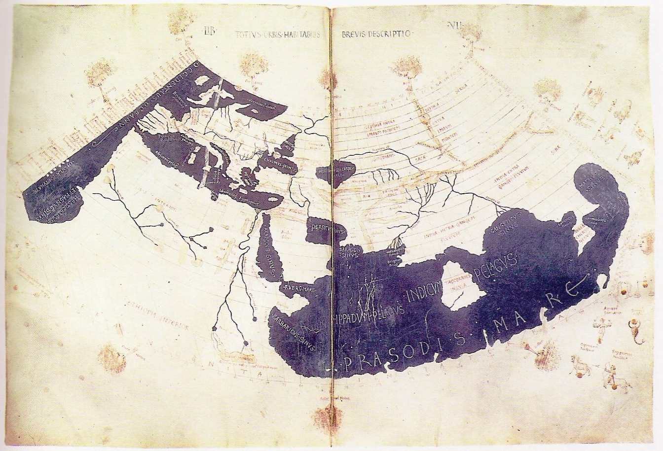
Ptolemy developed a system of latitude and longitude for mapping the world. His map covered 1/4 of the globe and was the standard until the Renaissance.
Find a long pole and use it to measure the angle of the sun with respect to due south. Take the measurement at the moment when the sun is highest in the sky. Use a pendulum bob to ensure that the pole is precisely vertical. At the same time, have an accomplice at a different latitude perform the same measurement. Use Google maps to determine the distance between you and your accomplice in the North-South direction, and use the measurements to calculate the radius of the Earth.
The radius of the Earth is
θ1 =  Angle of the shadow measured in New York City in degrees
θ2 =  Angle of the shadow measured by the accomplice
X  =  Distance between you and your accomplice in the latitude direction
   =  EarthRadius * |θ1-θ2| π / 180        (meters)

New York City Latitude   =  40.667 degrees North
New York City Longitude  =  73.933 degrees West
Earth radius             =    6371 km
Montreal and Manhattan have nearly the same longitude, which means that Montreal is directly north of Manhattan.
Manhattan latitude                     =  40.667 degrees North
Manhattan longitude                    =  73.933 degrees West
Earth radius                           =  R  =  6371 km
Montreal latitude                      =  45.500 degrees North
Montreal longitude                     =  73.567 degrees West
Montreal-Manhattan latitude difference =  θ
Montreal-Manhattan distance            =  X  =  R θ
What is the difference in latitude between Montreal and Manhattan in radians?
 |
 |
 |
|---|---|---|
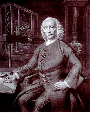
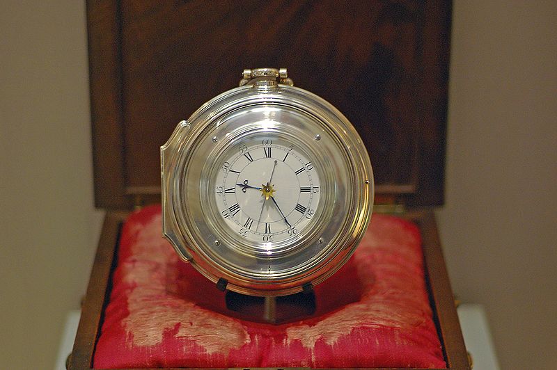
In 1714, the British Parliament established the "Longitude Prize" for anyone who could find an accurate method for determing longitude at sea.
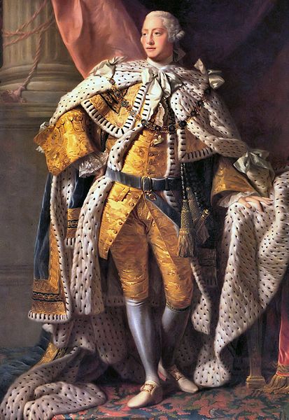
John Harrison solved the problem by developing precise clocks but Parliament refused to pay out. In 1772, Harrison gave one of his clocks to King George III who personally tested it and found it to be accurate to 1/3 of one second per day. King George III advised Harrison to petition Parliament for the full prize after threatening to appear in person to dress them down.
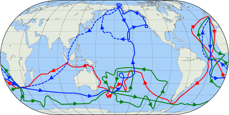
Maskelyne was the chairman of the board responsible for awarding the Longitude prize and he refused to award it to Harrison. Maskelyne developed the "Lunar distance method" for determing longitude, which was decisively defeated by Harrison's clocks in a test at Barbados. Also, James Cook abandoned the lunar distance method after his first world voyage and used Harrison's clocks for his 2nd and 3rd voyages.
From Wikipedia: "Cook's log is full of praise for the watch and the charts of the southern Pacific Ocean he made with its use were remarkably accurate."
Maskelyne held the post of "Astronomer Royal" and was hence in charge of awarding the Longitude Prize. He opposed awarding it to Harrison and Harrison was instead paid for his chronometers by an act of parliament.
 |
 |
 |
|---|---|---|
Measure the time of sunset and also have an accomplice at a different longitude do the same measurement. Use the measurements to calculate the difference in longitude and use Google maps to find the exact value.
T1  =  Time that you measure for sunset in hours
T2  =  Time that your accomplice measures for sunset in hours
L1  =  Your longitude in degrees
L2  =  Your accomplice's longitude in degrees

15 * (T1 - T2)  =  L1 - L2
Build a scale model of the sun, Mercury, Venus, the Earth, and the Earth's moon, with sizes and distances to scale. Choose a length of at least 50 meters for the distance from the Earth to the sun. Use Wikipedia for numbers.
Construct a scale model of the following systems:
The Earth, the moon, and the L2 Lagrange point.
The Milky Way, the Large Magellanic Cloud, Andromeda, and M87 (galaxy at the center of the Virgo Cluster).
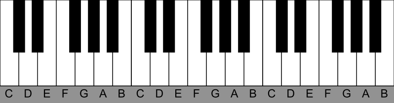
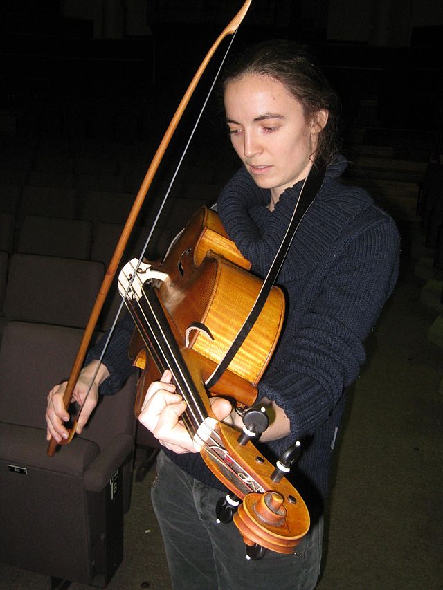
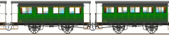
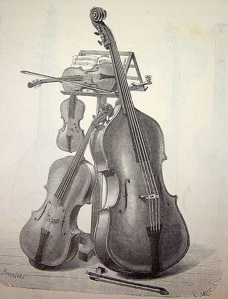
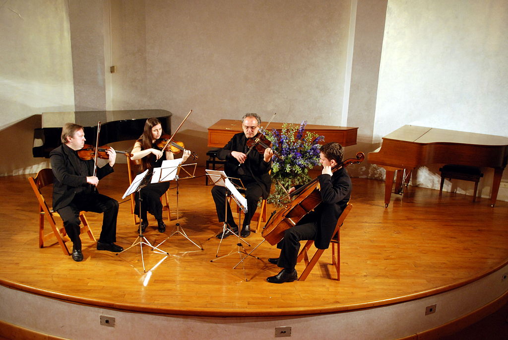
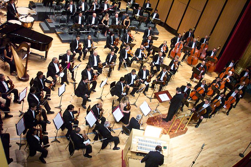
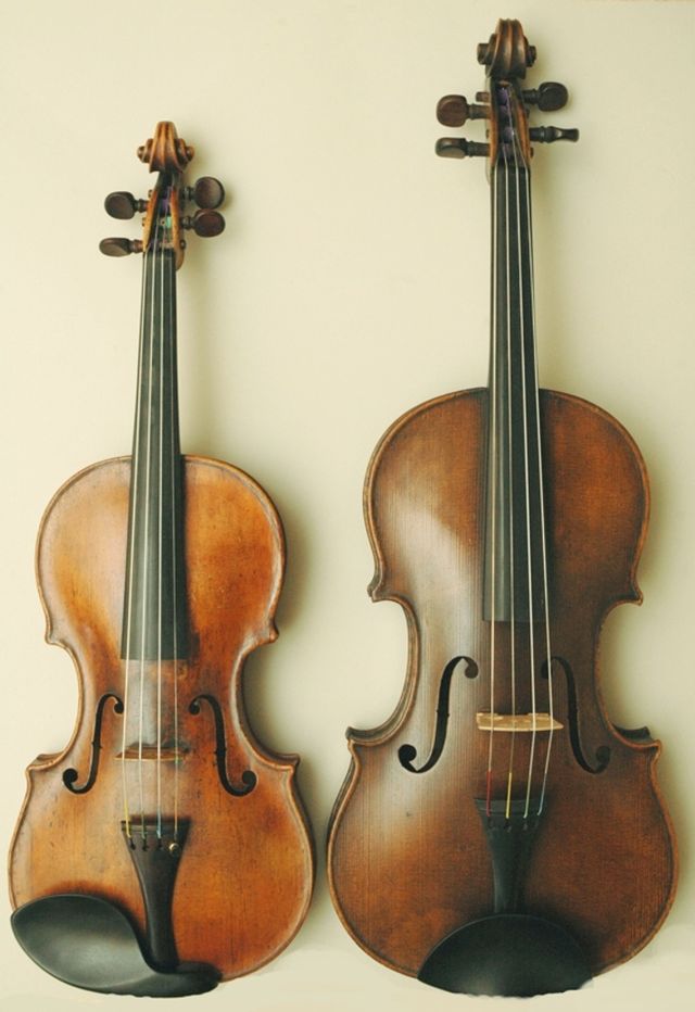
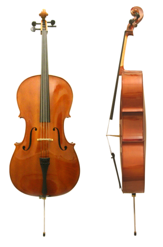
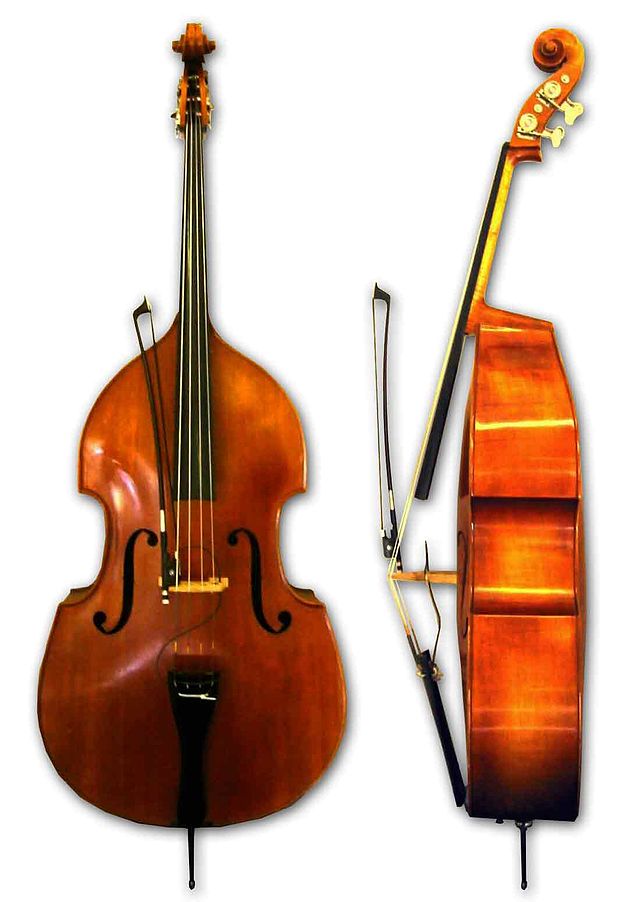
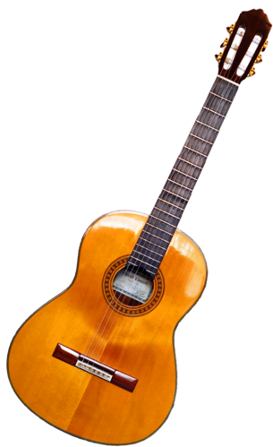
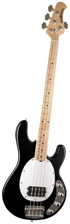
A violin, a viola, a cello, a bass, a guitar, and a bass guitar. Only size matters here, not distance.
 |
 |
|---|---|
 |
 |
|---|---|
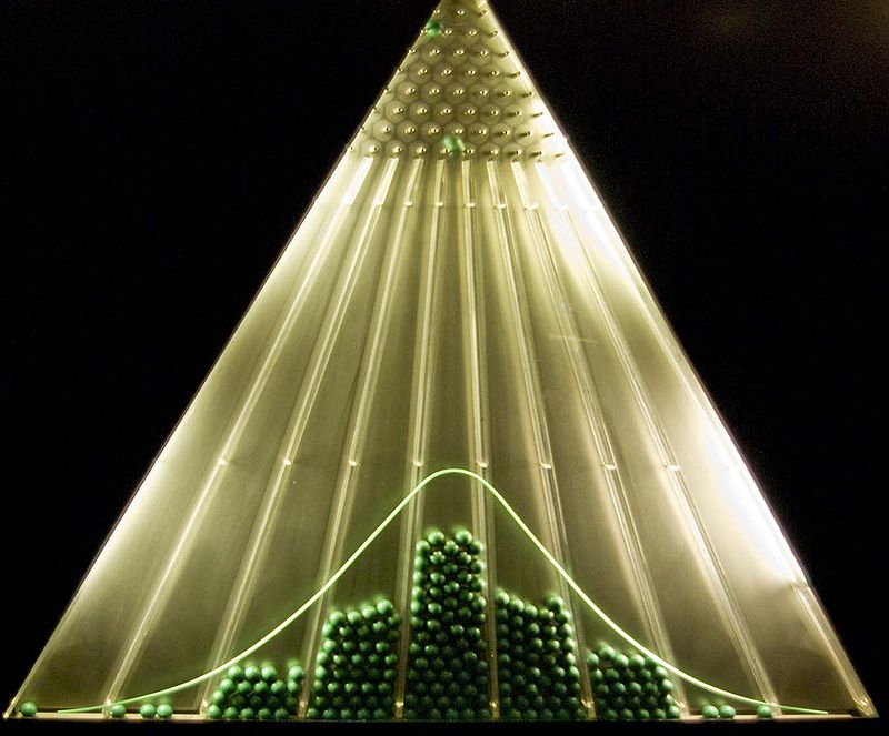
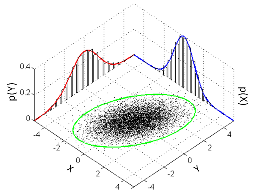
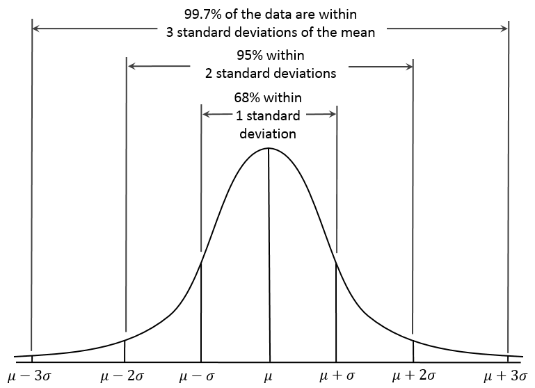
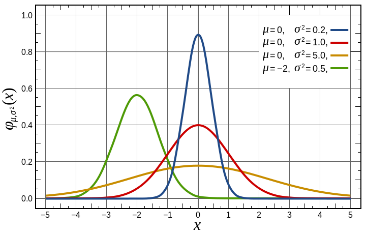
Suppose you have a set of measurements
Trial    Measurement
number     result

  1       1.232
  2       1.251
  3       1.256
  4       1.245
  5       1.233
  6       1.238
  7       1.433
The numbers cluster around the value "1.24" except for measurement #7 "1.433", which is an "outlier". Generally the outliers are removed and the error is computed from the well-baheaved numbers. Usually the outliers are errors, although on occasion it can turn out that the outlier is the correct measurement and the seemingly well-bahaved numbers are in error. There is no general rule for this. One has to be careful. In the following calculations we exclude the outlier.
Suppose we have N measurements Xj. The mean is
Mean = N-1 * ∑j Xj = (1/6) * (1.232 + 1.251 + 1.256 + 1.245 + 1.233 + 1.238) = 1.242The "Gaussian error" is
Error2   =  N-1 * ∑j (Xj - Mean)2
         =  6-1  * [  (1.232-1.242)2 + (1.251-1.242)2 + (1.256-1.242)2
                     + (1.245-1.242)2 + (1.233-1.242)2 + (1.238-1.242)2 ]
         =  .0090
If we were to include the outlier then it would dominate the calculation, rendering the other measurements meaningless.
The measurement is quoted as
Measured value  =  Mean  +-  Gaussian error
                =  1.242 +-  .0090
Suppose the length of an object is measured several times, with the results in meters being:
X1  =  2.553
X2  =  2.534
X3  =  2.536
X4  =  2.563
X5  =  2.541
X6  =  2.544
X7  =  2.560
X8  =  2.539
What is the mean and the Gaussian error? Plot the data to show how it is distributed.
Energy        =  E               (Joules)
Mass          =  M               (kg)
Volume        =  Vol             (m3)
Time          =  T               (seconds)     Time required for the battery to drain
Power         =  P   =  E / T     (Watts)       Power delivered by the battery
Energy/Volume =  Evol =  E / Vol
Energy/Mass   =  Emass=  E / M
Battery energies are often quoted in WattHours or AmpHours.
Voltage     =  V  =  3.7 Volts for a Lithium battery
Current     =  I                   (Current supplied by the battery in Amps)
Power       =  P  =  I V           (Power delivered by the battery in Watts)
1 WattHour  =  Energy associated with a power of 1 Watt for a duration of 1 hour
            =  Power           *  Time
            =  1 Watt          *  3600 Seconds
            =  1 Joule/second  *  3600 seconds
            =  3600 Joules
1 AmpHour   =  Energy associated with a current of 1 Amps for a duration of 1 hour
            =  Power                *  Time
            =  Current  * Voltage   *  Time
            =  1 Amp    * 3.7 Volts *  3600 Seconds
            =  13320 Joules
For example,
20 WattHours  =  20 Watts * 3600 seconds  =  72000 Joules

5.4 AmpHours  =  5.4 * 13320 Joules       =  72000 Joules
For a phone or tablet battery, use the printed value for
WattHours or AmpHours to calculate the energy.
Measure the mass and volume and calculate the energy/mass and energy/volume.
Data for batteries from Amazon.com.
                   Energy   Energy  Length  Width  Height   Energy  Energy   $   Energy/$
                   density   (MJ)    (m)     (m)    (m)      (Wh)    (Ah)         (kJ/$)
                  (MJ/m3)
Anker Astro E3      900      .137   136.9    67.3   16.5     10        2.7   22    6.2
Poweradd Pilot Pro  680      .426   185.4   121.9   27.9    118.4     32    130    3.3
Ravpower 23000      650      .306   185     124.5   20.3     85.1     23    100    3.1

1 kJ  =  103 Joules
1 MJ  =  106 Joules
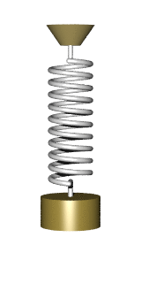
Force can be measured using mass and gravity.
Mass of an object                            =  M
Gravity acceleration at the Earth's surface  =  g  =  9.8 meters/second2
Gravity force at the Earth's surface         =  F  =  M g
A 1 kilogram object in Earth gravity exerts a force of 9.8 Newtons, which is 2.205 pounds.
 |
 |
|---|---|
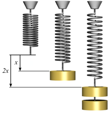
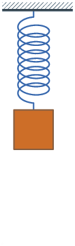
X     =  Length of a string under zero force
x     =  Change in string length when a force is applied
X+x   =  Total length of the string when a force is applied
K     =  Spring constant
Force =  Force on the spring
      =  K x      (Hooke's law)
Using any string or rope available, construct a plot of Force as a function of x,
all the way up to the breaking point. Set the string length "X" equal to 1 meter
if possible.
In the region of low x, what is the value of K?
 |
|---|
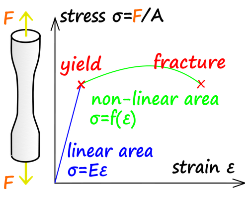
The elasticity of a wire depends on its intrinsic stiffness and on its cross sectional area.
The tensile modulus characterizes the stiffness of a wire and it is proportional to the spring constant.
For a wire,
X       =  Length of wire under zero tension force
x       =  Increase in length of the wire when a tension force is applied
K       =  Spring constant
Force   =  Tension force on the wire
        =  K x
Area    =  Cross-sectional area of the wire
Pressure=  Force / Area                  (Pressure, measured in Pascals or Newtons/meter2)
Strain  =  Fractional change in length of the wire     (dimensionless)
        =  x/X
Modulus =  Tensile modulus or "Young's modulus" for the wire material    (Pascals)
        =  Pressure / Strain
Starting from Hooke's law, we can derive an equation relating the modulus to the spring constant.
Force    =  Pressure * Area
         =  K * x
         =  K * X * x / X
         =  K * X * Strain
         =  Modulus * Area * Strain
Pressure =  (K * X / Area) * Strain
         =  Modulus * Strain
Modulus  =  K X / Area
K        =  Modulus * Area / X
 |
|---|
Choose a wire made out of any material, such as fishing line, a strip of duct
tape, or a shoelace. Hang the wire from the tower and add weights
to the wire until it breaks. Meaure and calculate the following:
If a force is applied to the center of a beam then it bends into a circular shape.
The tensile modulus and tensile strength can be measured by measuring the deflection.
Measure the following:
Plot the coefficient of friction as a function of sled mass.
Using fixed sled mass, plot the friction coefficient as a function of sled area.
The friction coefficient depends on the types of surfaces used.
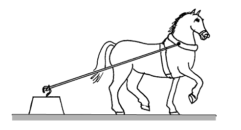
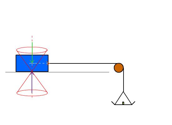
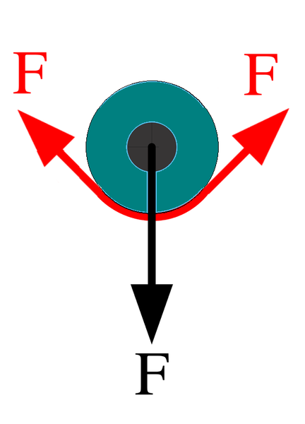
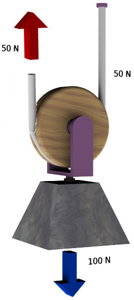
A pulley allows one to change the direction of a force.
This lab uses the
My Solar System simulaton at phet.colorado.edu.
Set up a simulation with the following parameters.
If the planet velocity is changed from the Y direction to the X direction, what is
Ve?
If the planet's X position is changed to 50 then what is
Vc?
If two planets are too close together then they will interfere gravitationally.
Using the simulator, set up a system with 2 planets.
Run the simulation for values of x ranging from 100 to 150 and determine
the minimum value of x for the planets to not interfere.
You can travel between planets with a "Hohmann maneuver". You start from the
inner circular orbit, fire the rocket, cruise on an elliptical "transfer orbit"
to the outer orbit, and then fire the rocket again to put the rocket into the
outer circular orbit.
The Earth and Mars system can be simulated using the following values.
Both the Earth and Mars are on circular orbits.
If Vlaunch is too low then the rocket won't make it to Mars.
If Vlaunch is too high then the rocket overshoots Mars' orbit.
This gets you to Mars faster but uses more fuel than the grazing orbit.
In the simulation, increase the Earth's "Y" velocity (Vtotal) until
you find the value that causes the Earth to graze Mars' orbit. What is this
velocity?
A planet "Tatooine" can be added halfway between Venus and Earth with
Using the
Lunar lander
simulation, try to land the spacecraft using a minimum of fuel.
What is the minimum fuel needed for a soft landing? Describe the strategy you used.
In the Android app "Osmos" you can experiment with maneuvering a spaceship in
a gravitational potential. Once the app is started go to level 3 "solar".
The game is like Saturn's ring. You are a snowball in the ring surrounded by
other snowballs and you can observe the differential motion between nearby
snowballs. You can also change your velocity and observe the effect on your
orbit.
If you are on a circular orbit of radius R and you want to change to a circular
orbit of radius 2R, what is the most efficient strategy? How would you draw a
diagram to illustrate this?
The game is also like a model of an accretion disk. In the sun's accretion
disk, objects accumulated by gravity into planets and the same thing happens in
Osmos. Large objects tend to accumulate faster than small objects and the end
result is a set of planets with widely-separated orbits. This phenomenon is
mirrored in Osmos because in the game, large objects tend to accumulate faster
than small objects.
Suppose you play the game with the purpose of observing how accretion works.
Move the spaceship to an orbit in the Kuiper belt so that it doesn't
interfere with the accretion. After the accretion has finished, what does the
result look like?
Film a ball rolling alongside a meter stick and analyze the video
frame-by-frame to evaluate time and position. For example,
The acceleration at Time=.50 can be approximated as:
Make a video of a ball rolling across a table and use the above procedure to generate a table
of positions, velocities, and accelerations.
Plot the following:
The drag force for an object moving through air is
For a falling balloon,
Add mass to the balloon so that its new mass is 4 times the old mass, and measure
the new terminal velocity. What is Q?
Suppose you want to estimate how far a soccer ball travels before air drag slows
it down. For a soccer ball,
Newton was also the first to observe the "Magnus effect", where spin causes
a ball to curve.
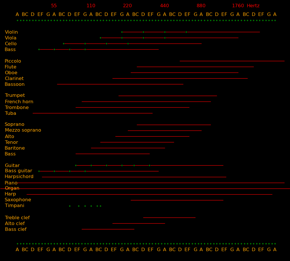
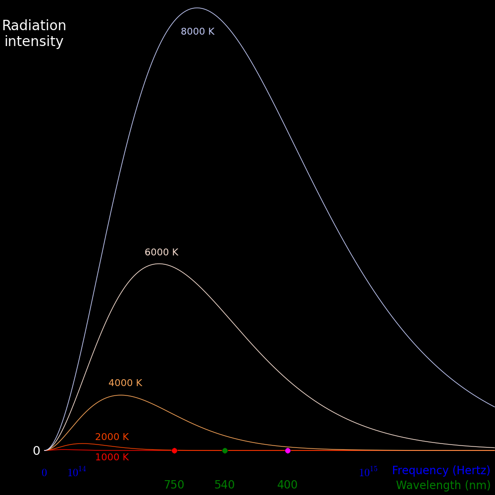
Humans can see light from 400 nm to 750 nm.
The Blackbody
radiation simualtion at phet.colorado.edu plots the blackbody spectrum as a function of
temperature. The area under the curve is the amount of energy produced by the blackbody.
You can subdivide the energy into bands. For example,
You can use the simulator to estimate the energy of each type by estimating the area under
the curve for the appropriate wavelength range.
In the figure above,
Estimate the temperature of a blackbody for which
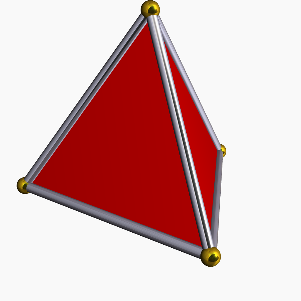
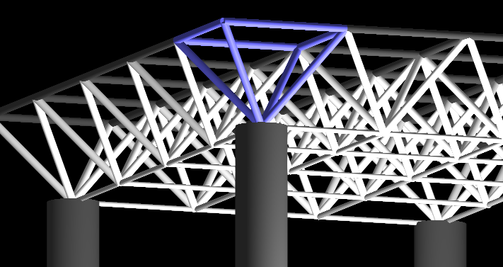
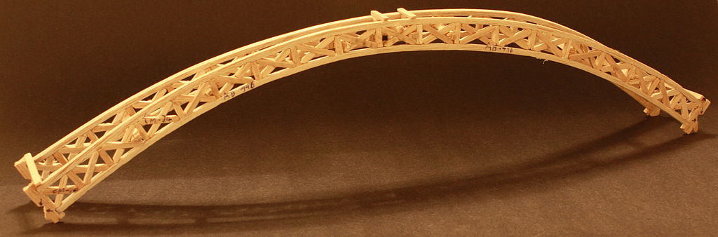
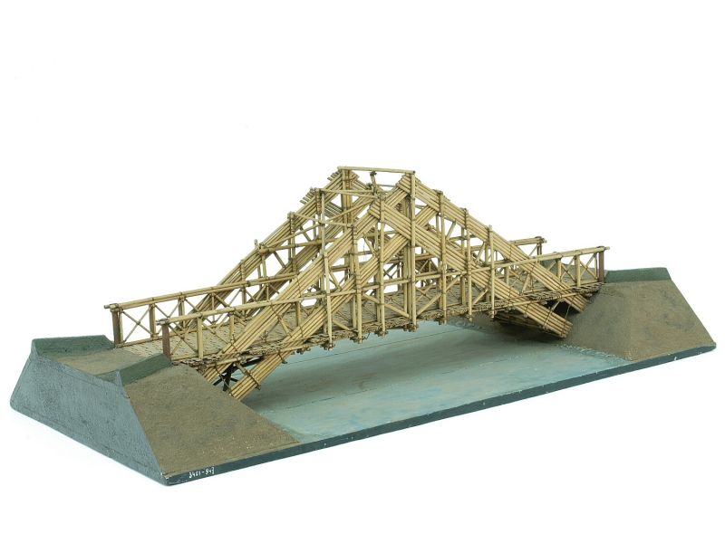
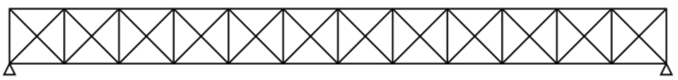
Build a bridge using the following materials:
To test the bridge, two tables will be placed 30 cm apart and the bridge will
be placed across the gap. Masses will be loaded on the bridge until it
breaks, and the score is the breaking is given as follows.
Build a tower 30 cm high. Weights will be placed on the tower until the tower
collapses and the score will be calculated similarly as the bridge score.
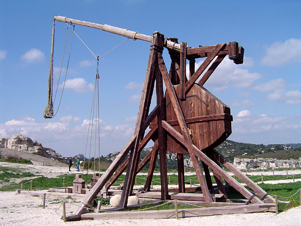
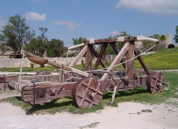
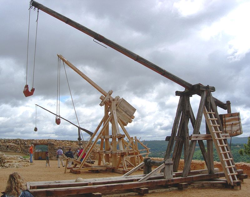
Build a catapult (trebuchet) to launch a projectile. You can design the
catapult so that it launches the projectile when a string is cut.
A catapult consists of a beam to support the masses, and a tower to support the beam.
The beam should be as long as possible and the tower should be as high as possible,
and both should be lightweight so that they can be carried by horses by a medieval army.
The drive mass is typically much larger than the projectile mass.
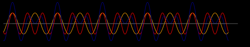
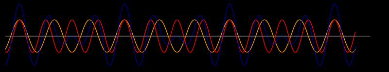
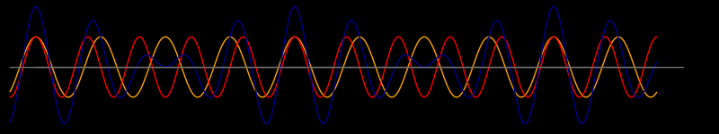
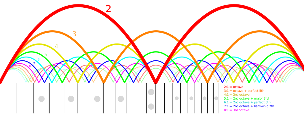
The properties of a wave are
A wave on a string moves at constant speed and reflects at the boundaries.
For a violin A-string,
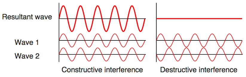
If a wave is linear then waves add linearly and oppositely-traveling waves
pass through each other without distortion.
If two waves are added they can interfere constructively or destructively,
depending on the phase between them.
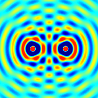
If a speaker system has 2 speakers you can sense the interference by
moving around the room. There will be loud spots and quiet spots.
The more speakers, the less noticeable the interference.
Noise-cancelling headphones use the speakers to generate sound that cancels
incoming sound.
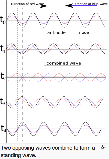
Two waves traveling in opposite directions create a standing wave.
Waves on a string simulation at phet.colorado.edu
For example, the overtones of an A-string with a frequency of 440 Hertz are
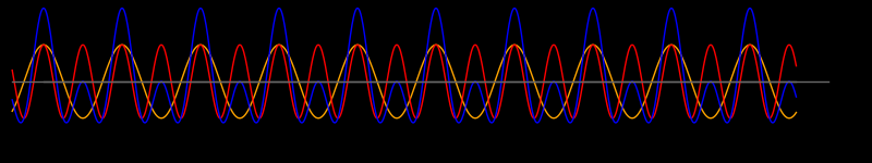
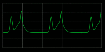
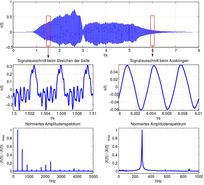
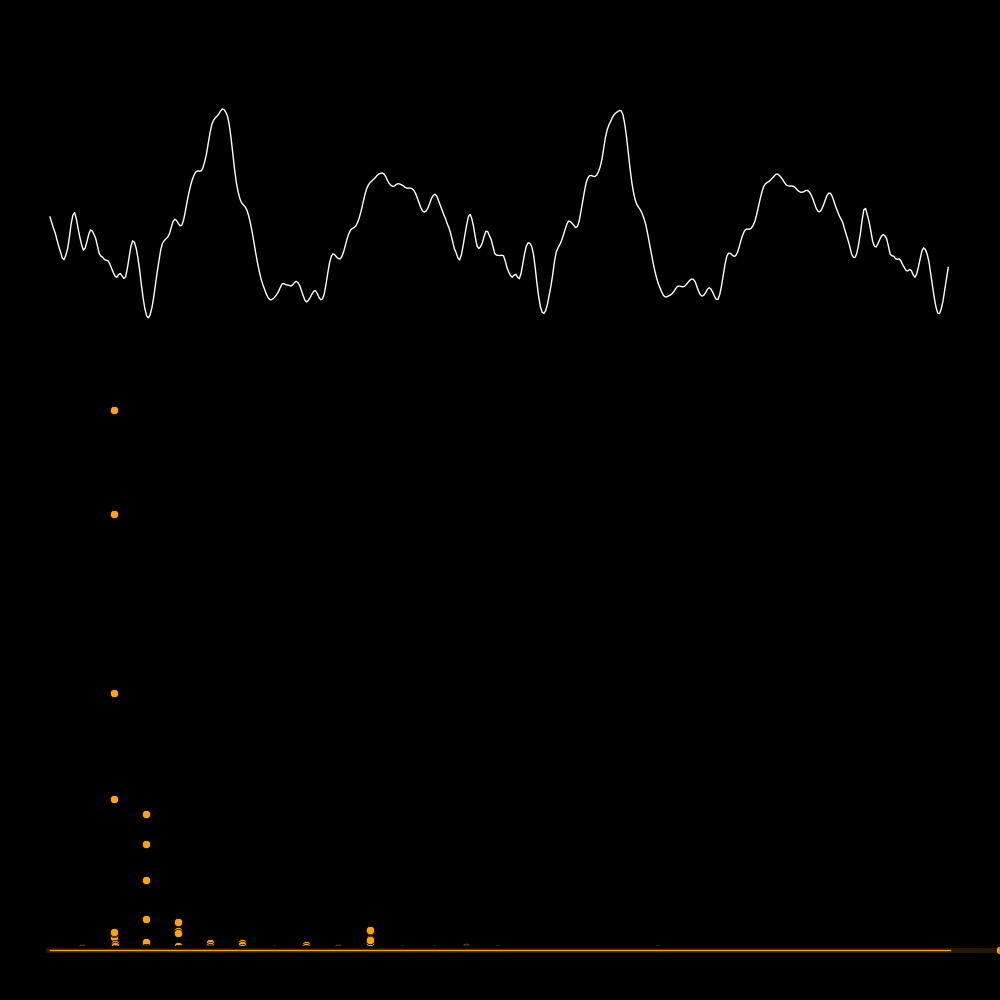
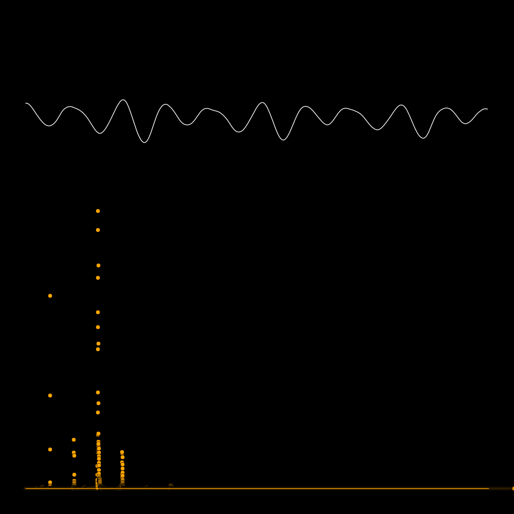
A spectrum tells you the power that is present in each overtone.
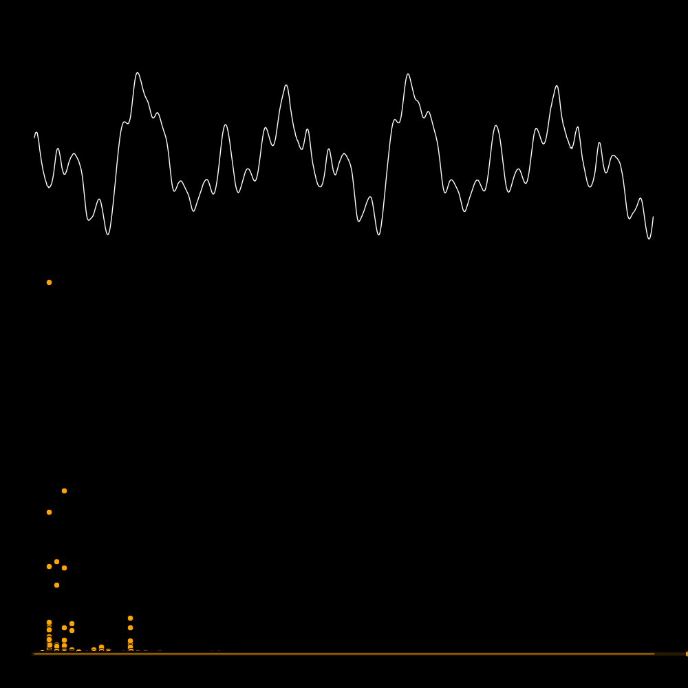
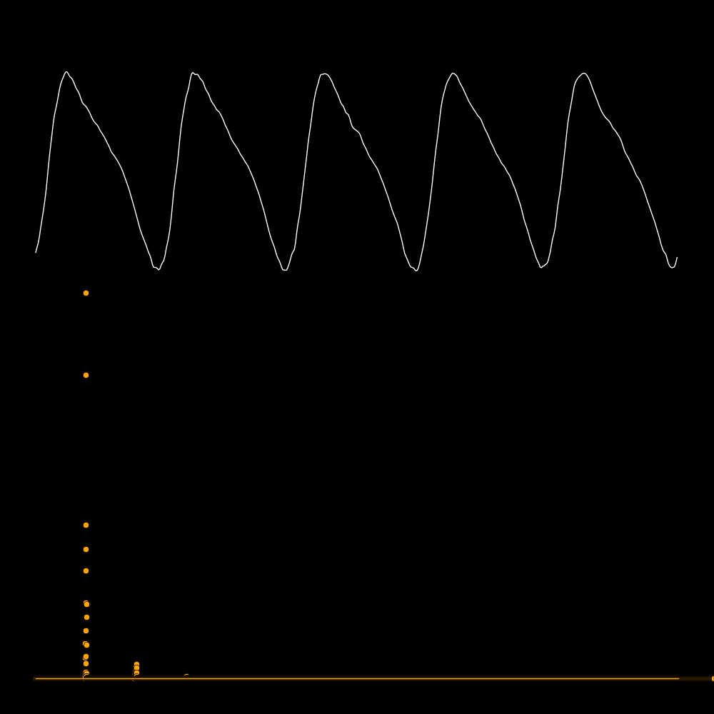
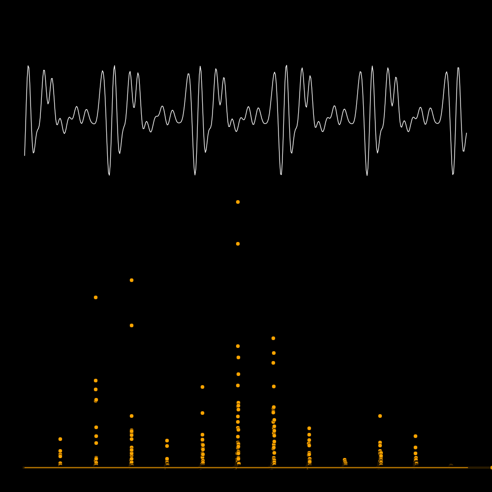
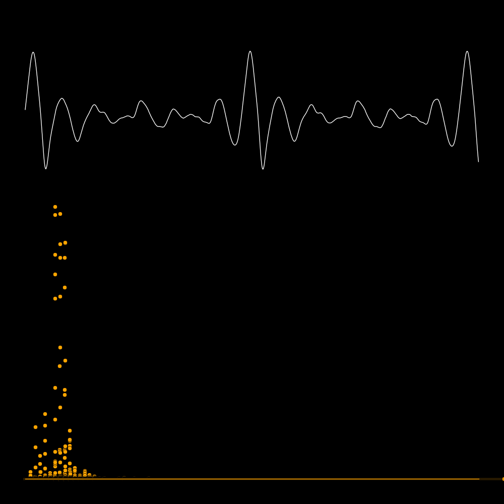
The first row is the waveform, the second row is the waveform expanded in time,
and the third row is the spectrum. The spectrum reveals the frequencies
of the overtones. In the panel on the lower left the frequencies are 300, 600, 900,
1200, etc. In the panel on the lower right there are no overtones.
A quality instrument is rich in overtones.
A waveform can be represented as an amplitude as a function of time or as an
amplitude as a function of frequency. A "Fourier transform" allows you to go
back and forth between these representations. A "spectrum" tells you
how much power is present at each frequency.
Fourier transform simulation
at phet.colorado.edu
Software such as "Garage Band", and the Android app "FrequenSee" can record music and
display the spectrum.
Every instrument produces sound with a different character. The sound can
be characterized either with the waveform or with the spectrum
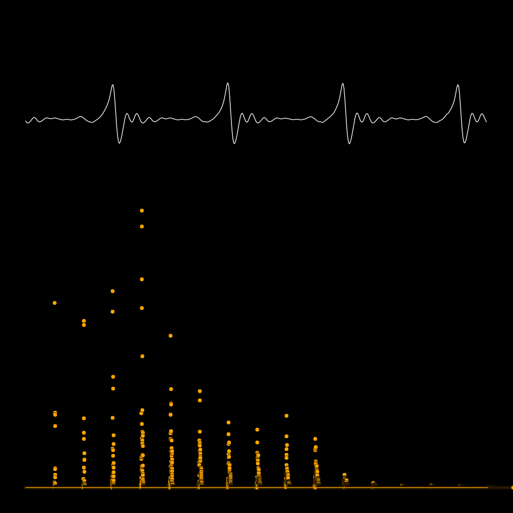
In the following plots the white curve is the waveform and the orange dots are
the spectrum.
Obtain a spectrum app for your phone. "FrequenSee" works for Android and
"Garage Band" works for iPhone. Find any 1D resonator (such as a pitchfork, a
string, or a bottle) and strike it so that it rings. Use the spectrum app to measure
the resonant frequencies. The resonant frequencies will appear as spikes in
the spectrum. Measure as many spikes as you can.
Try the experiment with different kinds of resonators. Use any resonator you can find.
1D resonators: Strings, rods, and bottles.
A wave on a string moves at constant speed and reflects at the boundaries.
For a violin A-string,
Build a musical instrument using rubber bands for strings. Invent a mechanism
for tuning the strings, such as like the pegs on a violin.
Give the instrument two identical strings and tune them to have the same frequency.
Measure the length and frequency of the string and calculate the wavespeed.
The frequency should be at least 200 Hertz to produce a useable tone.
Suppose you play the left string open and the right string with a finger down.
Try all possible values of R from 1 to 4 and look for harmonious values. Record any values
you find.
If you have an actual stringed instrument, try the experiment with the instrument.
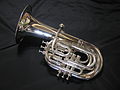
If you have a wind or brass instrument then try playing it together with another instrument.
An electrical pickup device will be provided (costs $2 at Radio Shack)
that can deliver the sound to a speaker, which will help in hearing the tone.
This allows lower frequencies to be used.
Build a musical instrument, either acoustic or electric (electrical pickups
will be provided). If it is acoustic, try to make the instrument as loud as
possible, especially for low notes (it's a challange to make low notes loud).
If it is electric, try finding novel resonators and record the sound.
Conduct an experiment to measure the sensitivity of human frequency perception.
For example, suppose you use a sound generator to produce a frequency of 440
Hertz and then slowly change the frequency until you notice that the frequency
has changed.
Suppose you play a note with a frequency of "F" and slowly raise it to a higher
frequency "f".
Let θ be the characteristic angle for which you can sense the direction
of a sound.
For the experiment there is noisemaker and a listener.
The noisemaker makes a sound while the listener has his eyes closed. The listener
points to the direction he thinks the sound is coming from, then opens his eyes
and measures the angle error. Do 6 trials to produce 6 numbers and then put these
numbers through the
error lab procedure to calculate the Gaussian error.
Obtain an Online tone generator.
Using a smartphone power spectrum app such as FrequenSee (Android) or Garage
Band (Apple), play a note at 220 Hertz and draw the power spectrum for various
speakers, such as:
Headphones
Using any speaker, start from a frequency of 440 Hertz and observe the peak of
the lowest-frequency overtone. Decrease the frequency and watch the peak. At
the moment it vanishes, record the frequency "Fbass".
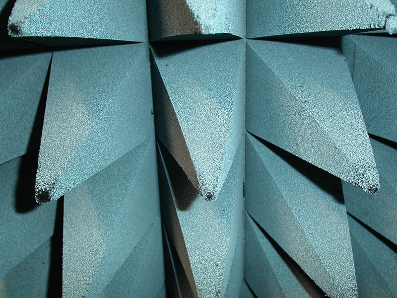
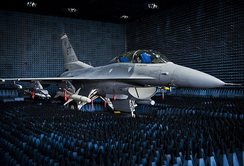
The walls of an anechoic chamber absorb all sound.
The absorbers are pointy to minimize the reflection of sound.
The information rate for sound is kilobytes/second and the rate for
vision is megabytes/second.
Build an anechoic chamber to be as silent as possible and measure the decibel
level. What measures did you have to take to reduce noise?
Obtain an app for measuring sound intensity and perform measurements in
any place you might be in Manhattan. Record the results.
Is there any place other than Central Park where you can't hear cars?
Use the app to measure the decibel reduction in sound when it passes through a wall.
Play a sound in an adjacent room and measure the sound level in the adjecent room and
the lab room.
Use a sound intensity app to measure the loudness of various instruments. Place
the microphone a standard 1 meter from the instrument for each instrument.
Measure the intensity of the lowest note and each octave above it.
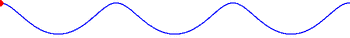
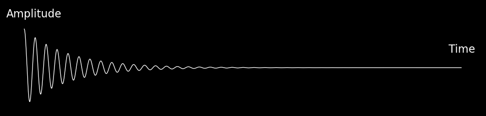
After a string is plucked the amplitude of the oscillations decreases with time.
The larger the damping the faster the amplitude decays.
For example, you can strike a resonator and estimate how long it rings before
damping out, or you can record the waveform with Garage Band and use it to
estimate Tdamp.
You can break a wine glass by singing at the same frequency as the glass's
resonanant frequency. An expensive wineglass has a large quality factor.
The larger the quality factor, the easier it is to break the glass by singing.
Get an account on Wikipedia and improve a page. Pages in need of improvement
include:
Greenhouses: Water and fertilizer requirements for crops.
Water quality of rivers, expressed as "Biological oxygen demand".
Sewage treatment: costs, fertilizer yield, biomass yield.
Irrigation: Data on water requirements with and without drip irrigation.
Seawater greenhouses: Data from existing greenhouses.
Desalination: Data from existing plants.
Emergency management: Disaster risk and monetary losses. Cost of prevention.
Iron fertilization of the oceans.
Urban forestry: Data for tree growth rates, trunk size, and height.
Solar cells: prices, efficiencies, and element requirements.
Wind turbines: prices, efficiencies, and element requirements.
Electric power distribution.
Prefabricated homes: Data for sizes, prices, and raw materials.
Patents: cost of solar cells, wind turbines, and smartphones.
Any topic relating to the presidential election.
Any topic from the history of science.
"The Hum"
Length of the wire under zero weight        =  X
Length change of the wire at breaking point =  x         Change in length required to break wire
Cross sectional area of the wire            =  A
Hanging mass required to break the wire     =  M
Gravity constant                            =  g  =  9.8 m/s2
Force required to break the wire            =  F  =  M g
Spring constant                             =  K     =  F / x
Tensile stiffness                           =  Pstiff =  F X / (x A)       (Pascals)
Tensile flexibility                         =  Tflex  =  x / X
Tensile strength                            =  Pstrong=  F / A             (Pascals)
Energy per volume of the wire material      =  e     =  ½ Pstiff T2flex       (Joules/meter3)

1 Pascal  =  1 Newton/meter2  =  1 Joule/meter3
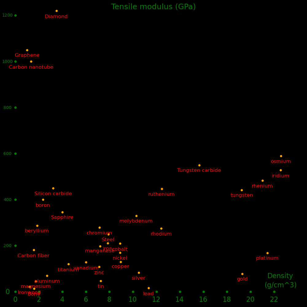
           Tensile  Breaking Breaking Tough  Tough/   Brinell  Density
           modulus  pressure strain          density  (GPa)    (g/cm3)
            (GPa)   (GPa)             (MPa)  (J/kg)

Beryllium    287     .448   .0016     .350     189       .6     1.85
Magnesium     45     .232   .0052     .598     344       .26    1.74
Aluminum      70     .050   .00071    .018      15       .245   2.70
Titanium     120     .37    .0031     .570      54       .72    4.51
Copper       130     .210   .0016     .170      19       .87    8.96
Bronze       120     .800   .0067    2.667     300              8.9
Iron         211     .35    .0017     .290      37       .49    7.87
Steel        250     .55    .0022     .605      77              7.9
Stainless    250     .86    .0034    1.479     185              8.0
Chromium     279     .282   .00101    .143     199      1.12    7.15
Molybdenum   330     .324   .00098    .159      15      1.5    10.28
Silver        83     .170   .0020     .174      17       .024  10.49
Tungsten     441    1.51    .0037    2.585     134      2.57   19.25
Osmium       590    1.00    .0018     .893      40      3.92   22.59
Gold          78     .127   .0016     .103       5.3     .24   19.30
Lead          16     .012   .00075    .045     3.8     .44     11.34

Rubber          .1   .016
Nylon          3     .075   .025     .938     815              1.15
Carbon fiber 181    1.600   .0088   7.07     4040              1.75
Kevlar       100    3.76
Zylon        180    5.80                                       1.56
Nanorope   ~1000    3.6     .0036      6.5    4980             1.3
Graphene    1050  160       .152   12190  12190000             1.0

Glass         45     .033                                      2.53
Concrete      30     .005                                      2.7
Granite       70     .025                                      2.7
Marble        70     .015                                      2.6

Bone          14     .130   .0093     604     377              1.6
Ironwood      21     .181   .0086     780     650              1.2
Human hair           .380
Spider silk         1.0                                        1.3
Sapphire     345    1.9     .0055    5232    1315              3.98
Diamond     1220    2.8     .0023    3210     920     1200     3.5


Toughness            =  Energy / Volume
Toughness / Density  =  Energy / Mass
A climbing rope should have a large toughness/density. It should absorb a lot of
energy and it should be light enough to carry.
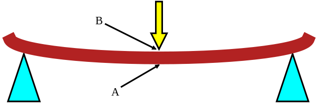
Length of the beam               =  X              (largest dimension of the beam)
Width of the beam                =  Y
Height of the beam               =  Z              (parallel to the force applied)
Force required to break the beam =  F              (at center of beam and in the direction of the Z axis)
Beam deflection when it breaks   =  x              (displacement of the center of the beam)
Spring constant                  =  K  =  F / x
Tensile modulus                  =  Y  =  (3/16) F X3 / (X Y x Z3)  =  (3/16) K X3 / (X Y Z3)
Internal strain when it breaks   =  S  =  4 Z x / X2
Tensile strength                 =  P  =  S Y      (internal pressure when it breaks)
Energy/Volume when it breaks     =  e  =  .5 * Y S2
Mass of the beam                 =  M
Density of the beam              =  D  =  M / (X Y Z)
Energy/Mass                      =  e / D
Gravity constant                            =  g  =  9.8 meters/second2
Mass of a sled resting on a table           =  Msled
Mass of a weight hanging from the wire      =  Mhang
Force of the sled on the table              =  Fsled  =  Msled g
Force on the weight hanging from the wire   =  Fhang  =  Mhang g
Area of the sled in contact with the table  =  A
Minimum sideways force to move the sled     =  Q Fhang
Coefficient of friction of the sled         =  Q  =  Fhang / Fsled  =  Mhang / Msled
Construct a sled and place masses on the sled. Attach a wire to the sled and
use the wire to generate a sideways force. Add weights on the wire until the
sled moves and measure the required weight. Calculate the friction
coefficient.
Surface   Surface         Friction
  #1        #2           coefficient

Concrete  Rubber            1.0
Steel     Steel              .8
Wood      Wood               .4
Metal     Wood               .3
Concrete  Rubber (wet)       .3
Wood      Ice                .05
Ice       Ice                .05
Steel     Ice                .03
Try experiments with different kinds of surfaces and measure the coefficient of friction.
         Mass     Position     Velocity
                    X    Y     X    Y

Body 1    100.      0    0     0    0      Star
Body 2      1.    100    0     0    V      Planet


Vc  =  Velocity for which the planet orbits as a circle.
Ve  =  Escape velocity.  Minimum velocity to escape.
Try varying V and using trial and error, estimate the vales of
Vc and Ve. What does the formula below predict?
R  =  Planet X coordinate
Vc =  Velocity for a circular orbit
Ve =  Velocity for escape
G  =  Gravity constant
   =  10000 for the simulator
A  =  Gravitational acceleration
M  =  Star mass
m  =  Planet mass
For a planet on a circular orbit,
Gravitational Force  =  Centripetal force
    G M m / R2       =  m Vc2 / R

Vc  =  (GM/R)1/2
For a planet to escape the star,
Gravitational energy  =  Kinetic energy
     G M m / R        =    .5 m Ve2

Ve  =  √2 * Vc  =  (2GM/R)1/2
         Mass       Position    Velocity
                     X    Y     X    Y

Body 1    100.       0     0     0    0      Star
Body 2       .01   100     0     0  100      Planet 1
Body 3       .01     x     0     0    v      Planet 2
To give Planet 2 a circular orbit, use
v  =  1000 / √x


 x     v

100   100
105    98
110    95
115    93
120    91
125    89
130    88
135    86
140    85
145    83
150    82
If "x" is close to 100 then the planets interfere
gravitationally, and if "x" is far from 100 the planets ignore each other.
![]()
![]()
        Mass         Position   Velocity
                      X    Y     X   Y

Body 1  100.          0    0     0    0    Sun
Body 2     .000219  100    0     0  100    Earth
Body 3     .000032  152    0     0   81    Mars
In a Hohmann maneuver a spaceship starts at the Earth and fires its rockets in the
Y direction, in the same direction as the Earth's velocity.
Vearth  =  Earth velocity
Vlaunch =  Departure velocity of the rocket with respect to the Earth
Vtotal  =  Total rocket velocity
       =  Vearth + Vlaunch
If Vlaunch has the right value then the rocket's orbit will graze Mars' orbit,
and this represents the minimum amount of fuel.
        Mass         Position     Velocity
                      X    Y     X   Y

Body 1  100.          0    0     0    0    Sun
Body 2     .000219   72    0     0  118    Venus
Body 3     .000303   86    0     0  108    Tatooine, a clone of the Earth that is closer to the sun
Body 4     .000303  100    0     0  100    Earth
Is this system stable? How large do you have to make the mass of the middle planet to make
the system unstable?
 Time   Position
 (s)      (m)

  .0      .000
  .5      .100
 1.0      .195
 1.5      .285
 2.0      .370
 2.5      .450
 3.0      .525
The velocity at Time=.25 can be approximated as
Velocity = Change in position / Change in time = (.100 - .000) / (.5 - .0) = .2 meters/second
The velocity at Time=.75 can be approximated as
Velocity = (.195 - .100) / (1.0 - .5) = .19 meters/second
Continuing, we can generate a table of velocities.
 Time   Position   Velocity
 (s)      (m)      (m/s)

  .0      .000
  .25               .20
  .5      .100
  .75               .19
 1.0      .195
 1.25               .18
 1.5      .285
 1.75               .17
 2.0      .370
 2.25               .16
 2.5      .450
 2.75               .15
 3.0      .525
From the table you can tell that the object starts out with a velocity of .20 and decelerates.
Acceleration = Change in velocity / Change in time = (.19 - .20) / (.75 - .25) = -.02 meters/second2
We can continue the procedure to produce a table of velocities and accelerations.
 Time   Position   Velocity   Acceleration
 (s)      (m)      (m/s)      (m/s2)

  .0      .000
  .25               .2
  .5      .100                 -.02
  .75               .19
 1.0      .195                 -.02
 1.25               .18
 1.5      .285                 -.02
 1.75               .17
 2.0      .370                 -.02
 2.25               .16
 2.5      .450                 -.02
 2.75               .15
 3.0      .525
Position as a function of time
Velocity as a function of time
Acceleration as a function of time
Object mass = M
Object area = A Cross-sectional area
Object velocity = V
Air density = d = 1.22 kg/m3
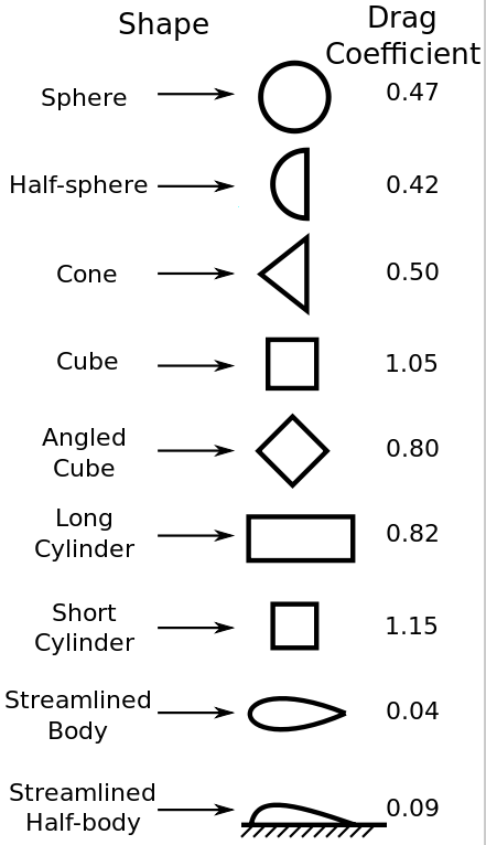
Drag constant = C Dimensionless and usually equal to 1
Drag force = F = .5 C d A V2
![]()
Gravitational acceleration         =  g    =  9.8 m/s2
Gravitational force on the balloon =  Fgrav =  M g
Air density                        =  d    =  1.22 kg/m3
Balloon cross-sectional area       =  A
Balloon velocity                   =  V
Balloon drag force                 =  Fdrag =  ½ C d A V2
Balloon drag coefficient           =  C    =  Fdrag / (½ d A V2)
Balloon terminal velocity          =  Vterm =  (2 M g / C / d / A)2
If a balloon is falling at terminal velocity then the gravitational force is equal to
the drag force.
Fgrav  =  Fdrag

M g   =  ½ C d A Vterm2
Drop a balloon and measure its mass, terminal velocity, and cross-sectional area.
Use the formula to calculate the drag coefficient.
Q = (Terminal velocity for mass "4M") / (Terminal velocity for mass "M")
Ball mass      =  M  =   .437 kg
Ball radius    =  R  =   .110 meters
Ball area      =  A  =  .0380 meters2  =  π R2
Ball density   =  D  =   78.4 kg/meter3
Air density    =  d  =   1.22 kg/meter3
Newton length  =  L  =    9.6 meters  =  M/d/A    Characteristic distance the ball travels before slowing down
Air mass       =  m  =    A L d                   Air mass that the ball passes through after distance L
Newton observed that the characteristic distance L is such that
m = M
Hence
L  =  M / (d A)
   =  (4/3) R D / d
The depth of the penalty box is 16.45 meters (18 yards). Any shot taken
outside the penalty box slows down before reaching the goal.
This plot shows the energy as a function of frequency emitted by a blackbody of various
temperature. Visible light ranges from the red dot to the magenta dot.
Type of light             Wavelength
                            (nm)
Threshold for cell damage   300
Magenta limit of vision     400
Magenta                     440
Blue                        480
Cyan                        520
Green                       555
Yellow                      620
Red limit of photosynthesis 680
Red                         700
Red limit of vision         750
Light is harmful if it has a wavelength smaller than 300 nm.
Photosynthesis can use light from 300 nm to 680 nm, except for the green light at 555 nm.
Energy           Largest     Smallest
type            wavelength  wavelength
                  (nm)         (nm)

Infrared        Infinity       750
Visual            750          400
UV                400            0
Total energy    Infinity         0
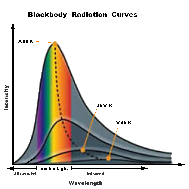

UV energy         =  Area of the gray area to the left
Visual energy     =  Area of the rainbow zone
Infrared energy   =  Area of the gray area to the right
The sun has a temperature of 6000 Kelvin. Using the simulator, estimate the values of
Infrared energy /  Total energy
Visual energy   /  Total energy
UV energy       /  Total energy
The estimate doesn't have to be overly precise. An eyeball estimate will do.
UV energy / Total energy = 1/100
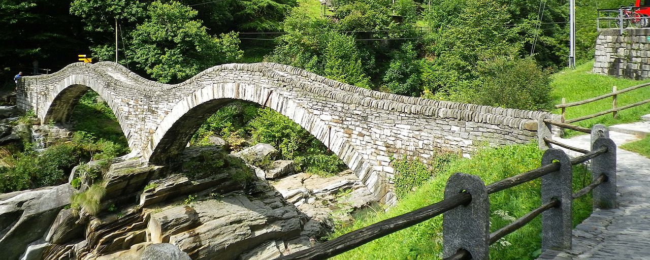
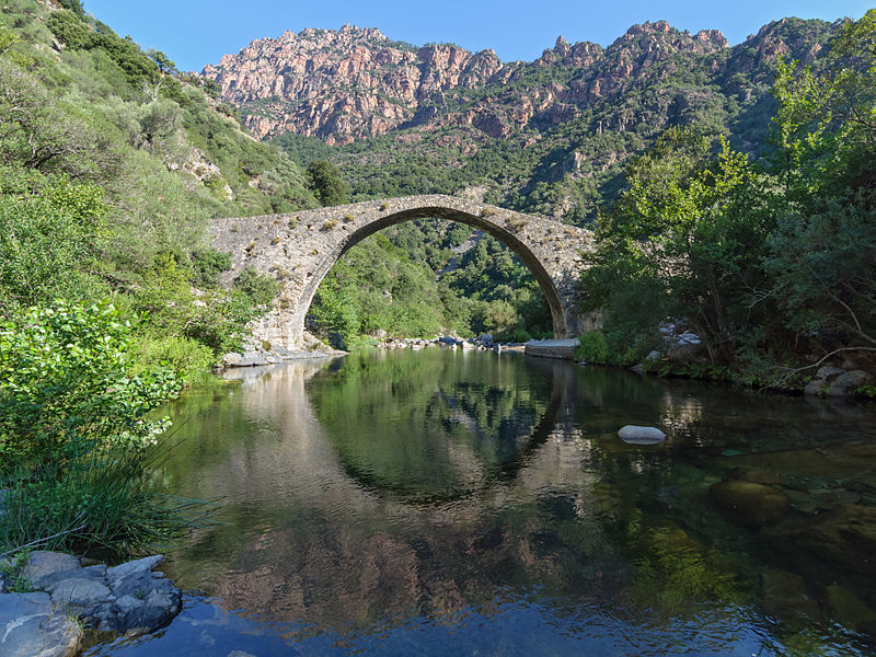

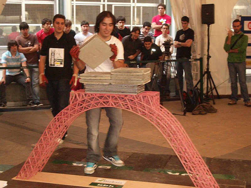
Wood (tongue depressor, toothpick, chopstick, etc.)
Paper (regular paper or file folder paper)
Superglue
Cotton string
Duct tape
Plastic straw
Mbreak  =  Mass required to break the bridge
Mbridge =  Mass of the bridge   (40 grams maximum)
S      =  Score of the bridge
       =  Mbreak / Mbridge
Mbreak  =  Mass required to break the tower
Mtower  =  Mass of the tower   (40 grams maximum)
S      =  Score of the tower
       =  Mbreak / Mtower
Mcat  =  Mass of the catapult  (40 grams maximum)
Mdrive=  Mass of the object used to drive the catapult  (can have any value)
Mproj =  Mass of the projectile launched by the catapult  (can have any value)
X    =  Distance the projectile travels, measured from the front of the catapult
S    =  Score of the catapult
     =  X Mproj


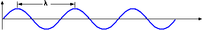
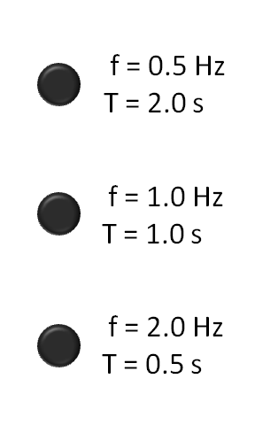
Frequency  =  F  (seconds-1)
Wavelength =  W  (meters)
Wavespeed  =  V  (meters/second)
Period     =  T  (seconds)  =  The time it takes for one wavelength to pass by
Wave equations:
F W = V

F T = 1
A train is like a wave.
Length of a train car =  W  =  10 meters         (The wavelength)
Speed of the train    =  V  =  20 meters/second  (The wavespeed)
Frequency             =  F  =  2 Hertz           (Number of train cars passing by per second)
Period                =  T  =  .5 seconds        (the time it takes for one train car to pass by)
Speed of sound at sea level    =  V  =  340 meters/second
Frequency of a violin A string =  F  =  440 Hertz
Wavelength of a sound wave     =  W  =  .77 meters  =  V/F
Wave period                    =  T  =  .0023 seconds

Frequency                           =  F  =  440 Hertz
Length                              =  L  =  .32 meters
Time for one round trip of the wave =  T  =  .0023 s  =  2 L / V  =  1/F
Speed of the wave on the string     =  V  =  688 m/s  =  F / (2L)

String equation:  2 L V = F

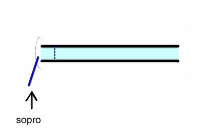
In a reed instrument, a puff of air enters the pipe, which closes the
reed because of the Bernoulli effect. A pressure pulse travels to the other
and and back and when it returns it opens the reed, allowing another puff of
air to enter the pipe and repeat the cycle.
Whan a wave on a string encounters an endpoint it reflects with the waveform
preserved and the amplitude reversed.
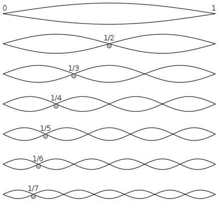
When an string is played it creates a set of standing waves.
Length of a string = L
Speed of a wave on the string = V
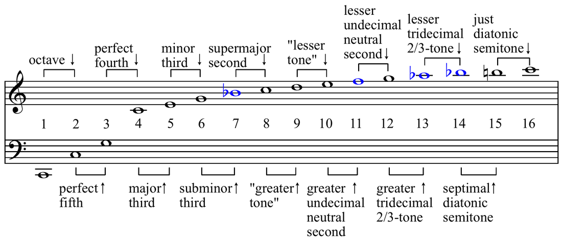
Overtone number = N An integer in the set {1, 2, 3, 4, ...}
Wavelength of an overtone = W = 2 L / N
Frequency of an overtone = F = V / W = V N / (2L)
N = 1 corresponds to the fundamental tone
N = 2 is one octave above the fundamental
N = 3 is one octave plus one fifth above the fundamental
N = 4 is two octaves above the fundamental
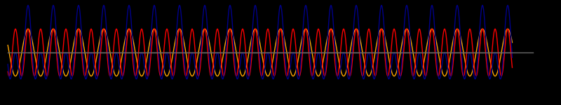
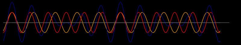
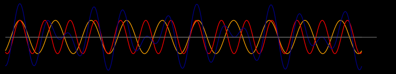
Audio: overtones
Overtone  Frequency   Note

   1         440       A
   2         880       A
   3        1320       E
   4        1760       A
   5        2200       C#
   6        2640       E
   7        3080       G
   8        3520       A
Overtone simulation at phet.colorado.edu
F1  =  Frequency of the lowest-frequanty spike
F2  =  Frequency of the spike with the next highest frequency after F1
F3  =  Frequency of the spike with the next highest frequency after F2
F4  =  etc.
R2  =  F2 / F1
R3  =  F3 / F1
R4  =  F4 / F1
Calculate R2, R3, R4, etc., for as many spikes as the
resonator has.
2D resonators: Drums, plates, the body of a stringed instrument.
3D resonators: Interior of a soccer ball or globe.
Frequency of the lowest-frequency overtone =  F  =           =  440 Hertz     (= F1 from above)
Length of the string                       =  L  =           =  .32 meters
Time for one round trip of the wave        =  T  =  2 L / V  =  1/F  =  .0023 s
Speed of the wave on the string            =  V  =  F / (2L) =  688 m/s

String equation:  2 L V = F
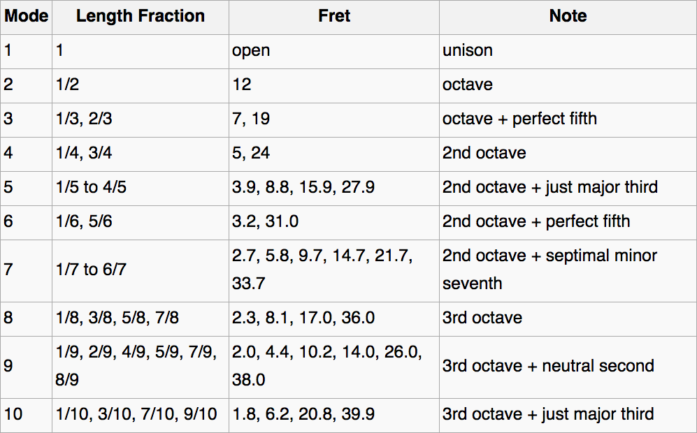
For each of the 1D resonators from the previous lab, measure the length of the
resonator and the frequency of the lowest-frequency note and use them to
calculate the wavespeed V.
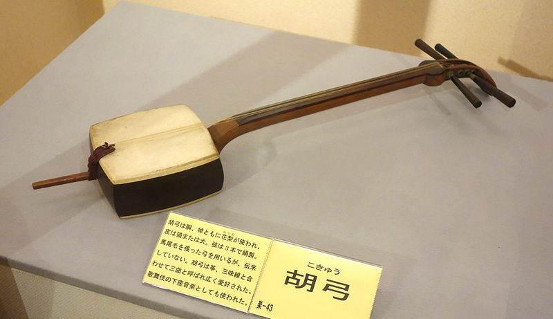
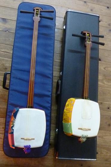
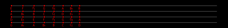
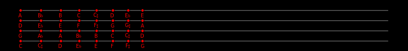
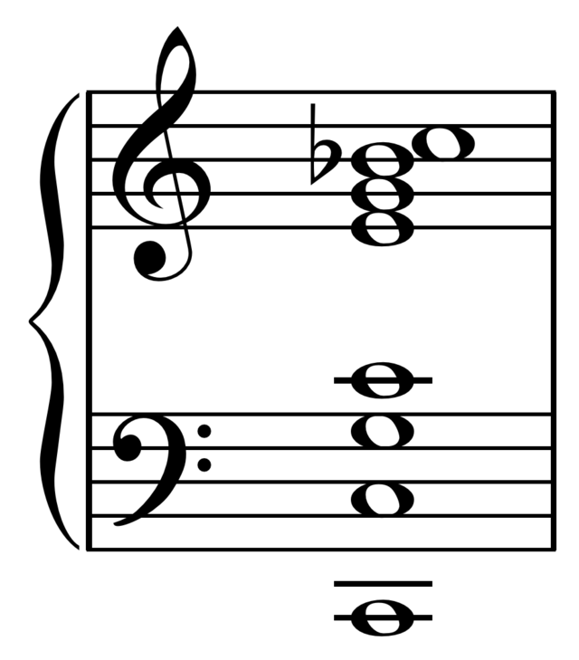
.jpg)
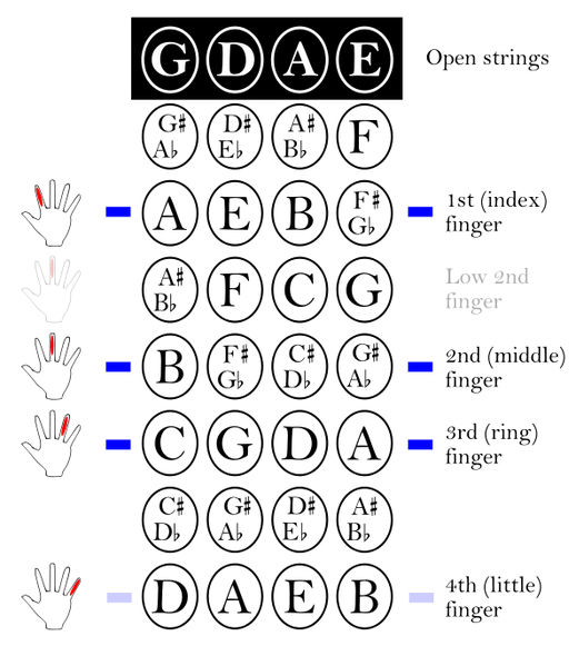
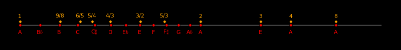
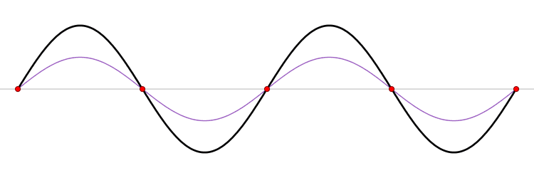
L1  =  Length of the open left string
L2  =  Length of the right string, from one end to the finger
      This is the active part of the string that can vibrate when you pluck it.
      L1 > L2
R  =  Frequency ratio between the two notes.
   =  L1 / L2
Pythagoras tried different values of R and found that some values sound harmonious
and others sound dissonant.
Original frequency          =  F  =  440 Hertz
Frequency sensitivity       =  Frez              Resolution for measuring a frequency of "F"
Frequency sensitivity ratio =  R  =  Frez / F    Relative frequency resolution that is independent of F
Online tone generator
If   |f-F|  <  Frez               then "f" sounds the same as "F"
If   |f-F|  >  Frez               then "f" sounds different from "F"
Conduct an experiment to measure the value of R for a range of frequencies F = 440
and 880 Hertz.
Smartphone
Tablet
Laptop
Desktop
The large speaker in the lab
Fbass  =  Lowest frequency that a speaker can produce
D     =  Diameter of the speaker
Measure Fbass and D for each of the speakers listed above.

F    =  Frequency of the string
T    =  Time for one oscillation of the string
     =  1/F
Tdamp=  Characteristic timescale for vibrations to damp
q    =  "Quality" parameter of the string
     =  Characteristic number of oscillations required for the string to damp
     =  Tdamp / T
     =  Tdamp * F
The smaller the damping the larger the value of q.
For most musical instruments, q > 100.
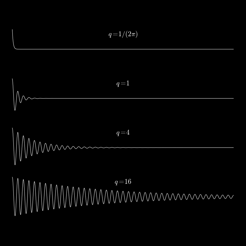
For various resonators, measure Tdamp and F and use them to estimate
the quality factor q = Tdamp F.
![]()
© Jason Maron, all rights reserved.