The Phurba algorithm for simulating magnetohydrodynamics
Way of the Intercepting Asymptote


* Phurba paper #1
* Phurba paper #2

"Phurbas: An Adaptive, Lagrangian, Meshless, Magnetohydrodynamics Code. I. Algorithm"  Maron, McNally & Mac Low, ApJS 2012, Vol 200, 1, 6
"Phurbas: An Adaptive, Lagrangian, Meshless, Magnetohydrodynamics Code. II. Implementation and Tests"  McNally, Maron & Mac Low. ApJS 2012, Vol 200, 1, 7

Particles vs. meshes
 |
 |
| Smoothed Particle Hydrodynamics |
Adaptive Mesh Refinement |
Algorithm classes
Phurba Pencil Riemann AREPO SPH Spectral
(AMR)
Geometry Particle Grid Grid Cell Particle Grid
Evolution Lagrange Euler Euler Lagrange Lagrange Euler
Space adapt Yes No Yes Yes Yes No
Continuous rez Yes No No Yes Yes No
Spatial fidelity 3rd order >6th order Riemann Riemann Poor Inf order
Conservative No No Yes Yes Yes No
Time fidelity D^2 / Dt^2 High Riemann Riemann Leapfrog High
Flexible PDEs Yes Yes No No No Yes
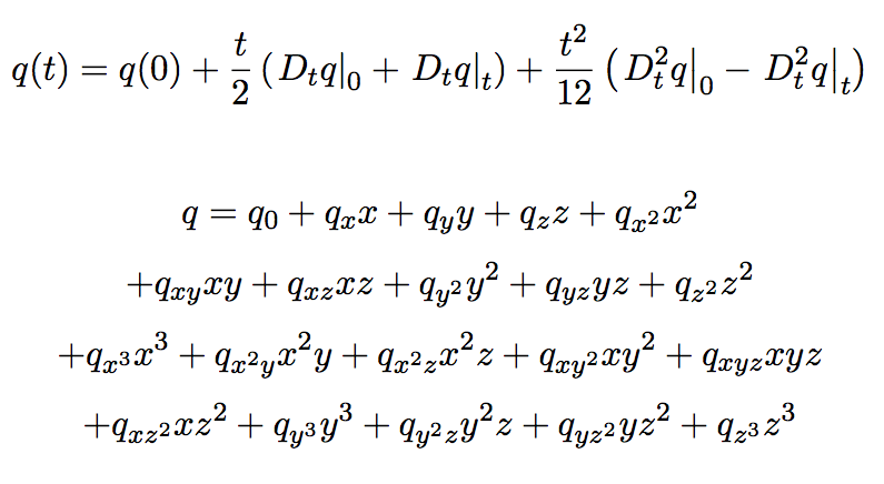
The Phurba algorithm is built from the principles of "Characteristic
(Lagrangian) evolution", "continuous fields", and "continuous spacetime
resolution". This gives it mathematical elegance and the flexibility to
simulate diverse classes of partial differential equations. This also makes it
impervious to the demons that haunt the Riemann and SPH algorithms.
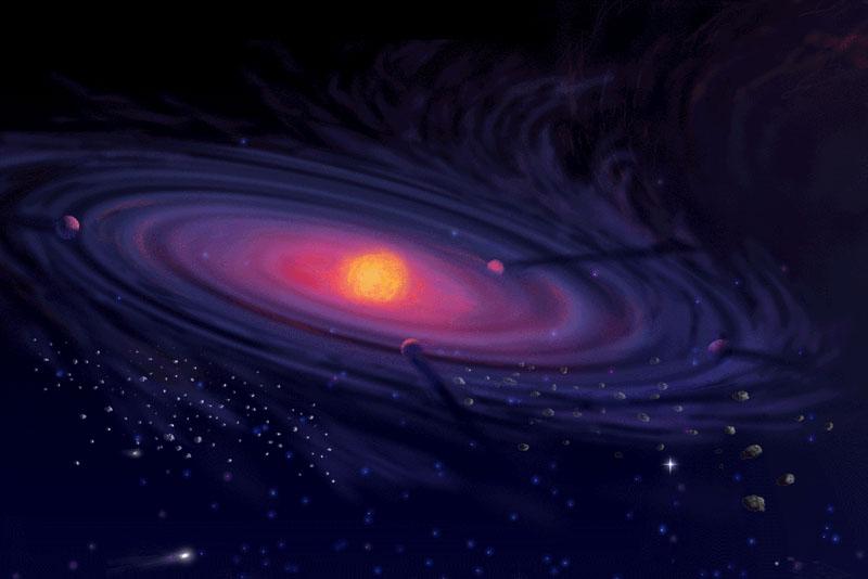
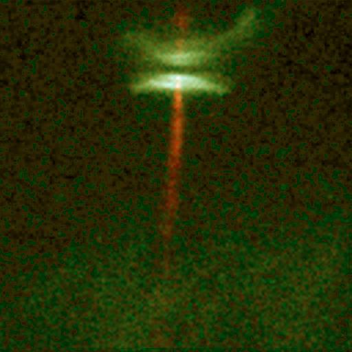
Phurba's flexibility is crucial for simulating complex objects such as a
planet-forming accretion disk.
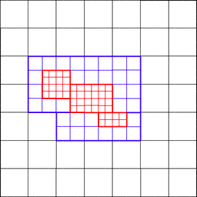
 Field values are carried on particles, which the phurba algorithm uses to construct
a continuous field profile. The construction is rubust for arbitrary particle
arrangements.
Field values are carried on particles, which the phurba algorithm uses to construct
a continuous field profile. The construction is rubust for arbitrary particle
arrangements.
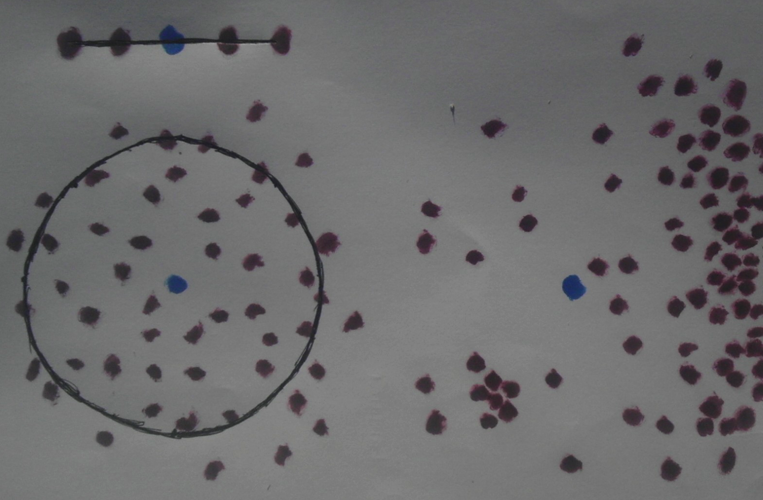
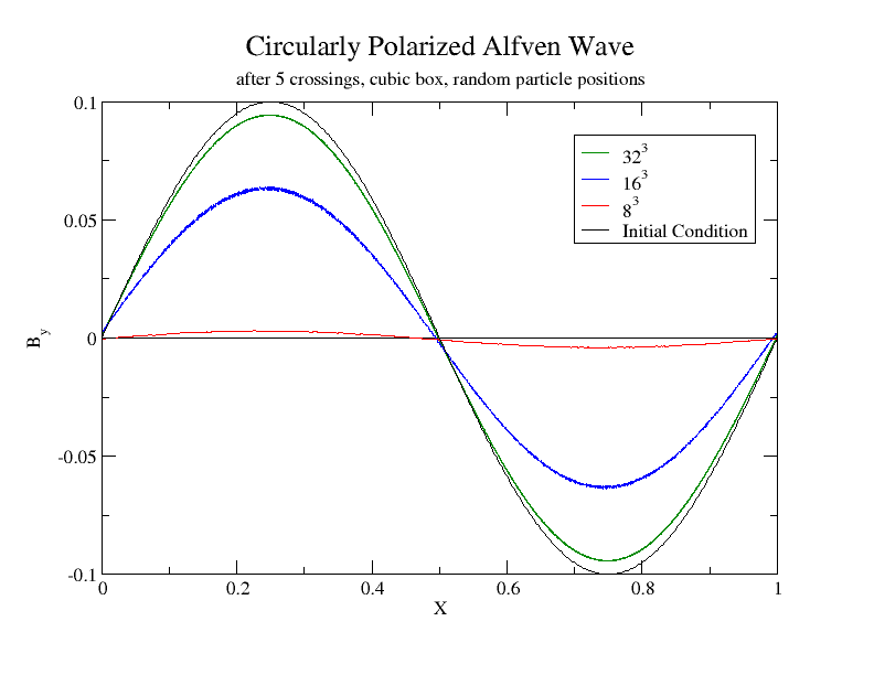 The phurba algorithm can simulate a high-resolution wave with a mere 8 particles.
To do this, SPH requires an order of magnitude more particles, plus inelegant
kludges.
The phurba algorithm can simulate a high-resolution wave with a mere 8 particles.
To do this, SPH requires an order of magnitude more particles, plus inelegant
kludges.
Time evolution and field construction